 Version 1:
Hi,
This is the archived webpage for my C++ tracer developed for CS 413 / CS 513 at the University of New Mexico, Fall 2011, presented very nearly as it appeared then (but now with various tweaks—mostly maintenance, a few updates, etc.). See also coursework and in particular newer raytracing results at the University of Utah.
There are pretty images here. I'm releasing them into the public domain, so if you want to use them as wallpapers, examples, textures, etc., you're completely free to do so. Might be nice to have some credit though :-)
Click a section below to expand:
Version 1:
Enough chit chat! Consider a scene file (the design of which is probably non-standard):
image {
    width 800
    height 600
    samples 1
}

camera {
    position 0.0 2.0 6.0
    center 0.0 0.0 0.0
    up 0.0 1.0 0.0
    image_plane 1.0
}

scene {
    object {
        position 0 0 0
        sphere {
            radius 1
        }
    }
    object {
        position 2 0 0
        sphere {
            radius 1
        }
    }
    object {
        position -2 0 -2
        sphere {
            radius 2
        }
    }
    object {
        position -2 -3 -2
        sphere {
            radius 1
        }
    }
    object {
        position -2 0 0
        sphere {
            radius 1
        }
    }
    object {
        position 2 2 0
        sphere {
            radius 1
        }
    }
    object {
        position 4 0 0
        sphere {
            radius 1
        }
    }
    object {
        position 4 0 2
        sphere {
            radius 1
        }
    }
}
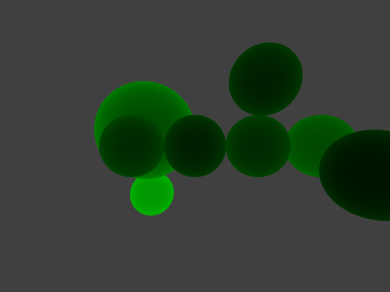
This[1] scene file will produce the an image like the following (click to enlarge):

The ray tracer can handle any number of spheres of any radius. Occlusion is handled properly. In this image, the spheres are colored by depth, with darker colors being closer surfaces and lighter colors being farther surfaces. Pressing "s" will save the image (if it is done rendering).
Version 2:
Added support for HDR rendering (just a few tweaks to the code). Right now, tonemapping isn't done (there's no need), but it could be easily added.
Also added stochastic supersampling. Taking n times as many samples per pixel of course slows down the rendering by a factor of n, but you can get very pretty images this way. Right now, it just uses uniform random samples over the pixel—nothing fancy like Poisson disk.
Most importantly, I added multithreaded rendering with any number of threads, fully integrated with tile-based rendering, for better cache coherency. The threads all work together to render the image. For the scene above, rendered with 10x10 pixel tiles and one sample per pixel, using one thread it takes 7.4 seconds. With two threads, 5.4 seconds. Because I'm testing on a dual-core architecture[2], performance goes down a little bit for each additional thread after two that I add. Also, the effect of the main thread should not be forgotten; limiting the framerate of the GUI improves render times significantly—perhaps 10–20%. A tile size of about 50x50 seems to be the best for performance. In the future, all render times will be with one thread unless expressed otherwise.
It was at this point that I began to restructure the code significantly. I completely rewrote the scene file parser (so it is much more robust and usable) using a tokenizer. This allowed me to support some nice syntax for some things, as well as giving better feedback about what syntax is acceptable. I put all the rendering stuff into its own class, and neatened things up a lot. I went bugsquishing, and killed a memory leak that occurred when closing the window in the middle of a render. I started making the raytracer compatible with glLibC, which I figured out how to turn into a library file.
I began to do some optimizations, and shaved a fraction of the second off the rendering time. But then, with both debug and release builds of the glLibC library available, I realized that I was now able to compile the program in release mode (i.e., compiler-optimized). 'Lo and behold, the program runs 30–50 times faster! The original image (with one sample per pixel) could now be rendered in 0.198 seconds, which is an interactive framerate! Keep in mind that this includes the overhead of the main thread drawing the scene intermediaries. A quick Google search shows that this is actually about the performance to be expected for a "realtime" CPU ray tracer.
This image at left was rendered using 2 threads and 50x50 tiles with 10 samples per pixel, in debug mode. It took about 56 seconds (about 10 times the cost of using one sample per pixel in debug mode). But, note the much smoother edges. The image in the middle was rendered using release mode and 100 samples per pixel. It renders in 9.69 seconds. The image at right was rendered using release mode and 1,000 samples per pixel. It renders in 99 seconds. Click to enlarge:

|

|
|
Clearly, you can see that it's a process of diminishing returns. The original image, with 1 sample per pixel, looks pretty bad, but even the image on the left, with just 10 samples per pixels, is good quality. There's noticeable improvement from 10 to 100 samples, but it's slight. The difference between 100 and 1000 samples is scarcely even perceptible.
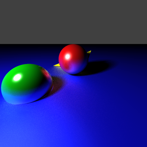
Okay, time to add some more primitives! I added planes and triangles, and set up lights and materials. Pop it all in the renderer with 100 samples per pixel with a new scenefile:
image {
    width 512
    height 512
    samples 100
}

camera {
    position 0.0 5.0 2.0
    center 0.0 0.0 0.0
    up 0.0 0.0 1.0
    image_plane 1.0
}

material "plane_material" {
    diffuse 0.05 0.05 1.0
    specular 0.2 0.3 1.0
    shininess 3
}
material  "sphere1_material" {   diffuse 1.00 0.05 0.05   specular 1. .9 .9   shininess  10   }
material  "sphere2_material" {   diffuse 0.05 1.00 0.05   specular .9 1. .9   shininess  30   }
material "triangle_material" {   diffuse 1.00 1.00 0.05   specular 1. 1. .9   shininess 100   }

light "light1" {
    color 1.0 1.0 1.0
    object:point {
        position 4 4 4
    }
}

scene {
    background 64 64 64
    object:sphere {
        use "sphere1_material"
        position 0 0 1
        radius 1
    }
    object:sphere {
        use "sphere2_material"
        position 2 2 0.2
        radius 1
    }
    object:plane {
        use "plane_material"
        position 0 0 0
        normal 0 0 1
    }
    object:triangle {
        use "triangle_material"
        position -1 -1 0.02
        position2 2 -2 .02
        position3 -1.5 -1.5 1.5
    }
}
. . . and in 6.75 seconds, you get the image below-right. The below-left image is an OpenGL rendering with 16x multisampling, for comparison. You'll notice that the results are very similar, while still being noticeably different. As an explanation, the ray tracer does all computations using double precision. Also, the spheres in the OpenGL rendering use 50 slices/stacks, while the raytracer's are mathematically perfect. OpenGL has a clipping plane, which was set to 5000.0, thus the blue plane primitive is not truly infinite. In any case, the point is to show that they're similar; I used the OpenGL rendering as a sanity check while working on the ray tracer.
|

|
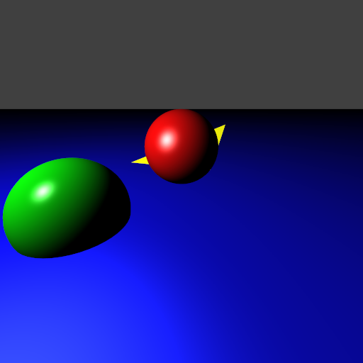
From here, I decided to add shadows. The change to the scene file is simple. I added:
action:shadow "light1" 1
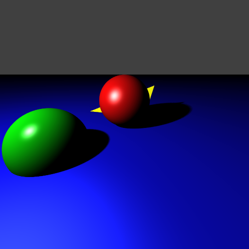
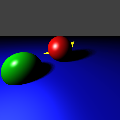
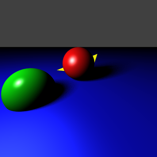
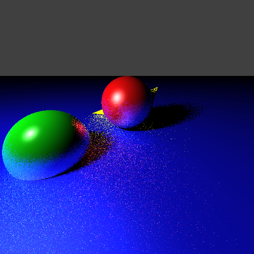
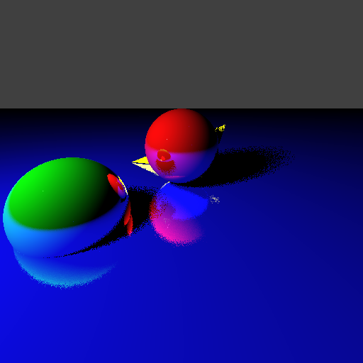
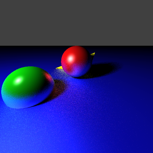
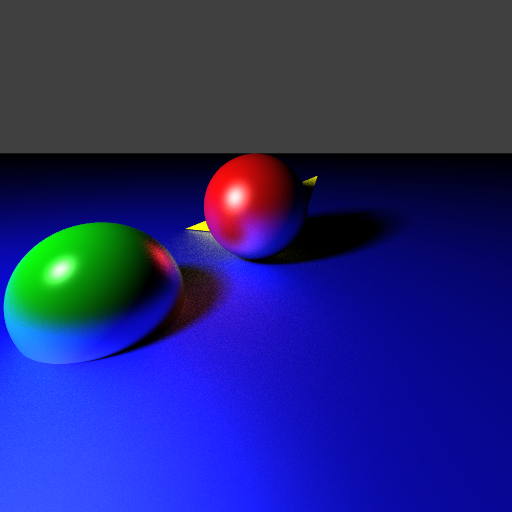
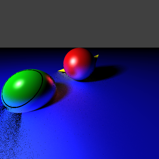
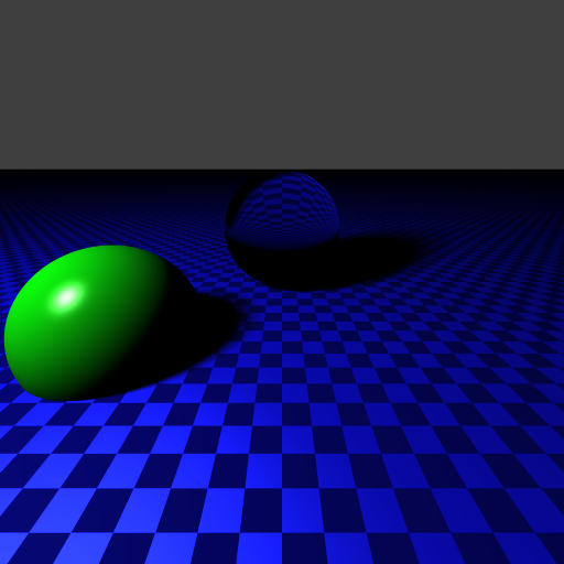
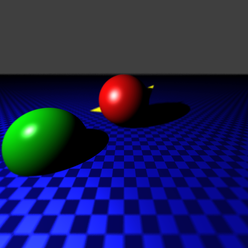
. . . under the material definition, which tells the renderer to send one random shadow ray toward light source "light1". Internally, it's more complicated than that! I split the intersection code into a separate method so that both the ordinary and the shadow casting code could use it. The result is the image below left (100 samples, 9.75 seconds). Notice that the shadow is completely black. This is because there is no ambient component in the materials. Adding one can be done by editing the scene file. Notice also that because the light's primitive is a point, the shadows are sharp. To soften things up a bit, I changed the light source to a sphere. The shadow rays are cast to a random point on the sphere/light. This approach called "distributed raytracing". The second, third, and fourth images were made with 10 samples per pixel, with each of those casting 10 random shadow rays, on light sizes of 0.1, 0.5, and 1.0, respectively. These three renders all took about 5½ seconds.

|
|
|
|
It should be noted that it's only the shadows here that have anything special done to them. The diffuse and specular lighting on the primitives still assume a point light source.
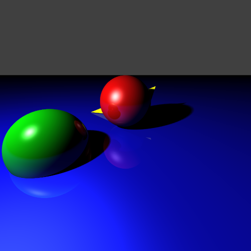
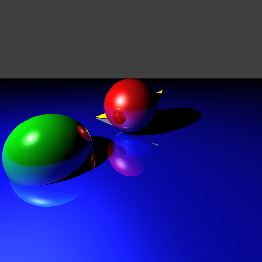
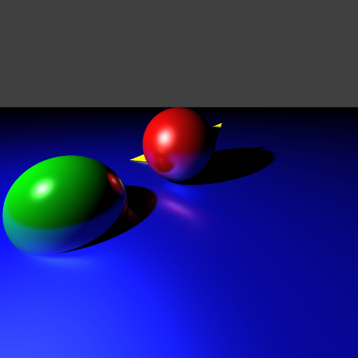
I then decided to add reflections. There was a bit of diciness, until I realized that in release mode, variables are not initialized. This resulted in a problem with my triangle intersection code. I fixed this, but there was was still noise in the image. I determined that this was due to the shadow and reflection rays being cast from the surface itself. I added an epsilon to the shadow and reflected rays' positions, and the problems disappeared. In the left and center pictures below, you can see the sharp reflections (10 pixel samples, 10 shadow samples (light radius 0.1), 1 reflection sample). They render in about 7½ seconds. The reflections are just added onto a pixel's color, being scaled (in the left by 0.2, on the right by 0.5).
I also added glossy reflection. This is a total hack, not really supported physically. It simply sends out a number of rays for each reflection vector. The result may be seen on the right (10 pixel samples, 10 shadow samples (light radius 0.1), and 10 reflection samples). Note that in the case of multiple reflection, it becomes exponential in the number of reflection rays processed. The render took 1 minute, 27 seconds.
|
|
|
For some reason, the rendering takes much longer when compiling on Linux. This is being looked into.
Version 3:
Version 3 revisits glossy reflections. I use a really lame method to get the samples, but at least it's accurate.
The initial attempt (below-left), with one sample per pixel, two reflection samples[3], one shadow sample, and a reflection coefficient of 1.0, took ~52 seconds to render.
|
|
This is good, but notice that it took 52 seconds! Clearly, this is unacceptable. Turned out that a hack that I had considered unimportant turned out to be important: to generate the samples, vectors with the proper random distribution were selected until a valid one was chosen (valid in this case means that the reflected ray didn't go into the surface). Note that this has an upper bound of infinity on the rendering time! Instead, when an invalid sample was chosen, it was flipped up above the surface, so it would then be valid. This resulted in essentially the same rendering, but at a much better 0.65 seconds (I redid the above left image with 1000X specular, resulting in above right image; it shows that the admittedly fuzzy result on the left is actually correct). With the inefficiency alleviated, the sample count could be bumped up.
Unfortunately, there were some problems. The most obvious was that the reflection vector's epsilon offset is being added to the unperturbed reflection vector. In practice, I think this is okay; the difference should be completely negligible.
The most annoying problem was that when the rays were allowed to recurse, the reflection gradually vanished. The result turned out to be that the rotation matrix used in the rotation was global, but they were being set in the recursive function. The day is saved! The image at left has one sample per pixel, ten reflection rays, ten shadow rays, coefficient 1.0, and took ~5 seconds to render. The one in the middle has ten samples per pixel, ten reflection rays, ten shadow rays, coefficient 1.0, and took about 1 minute 4 seconds to render. The one on the right has one hundred samples per pixel, ten reflection rays, ten shadow rays, coefficient 1.0, and took about 11 minutes, 5 seconds to render:
|
|

|
At this point, I did a slight optimization on the matrices, which unfortunately only shaved about 4 seconds off the rendering time of the above-middle image. This wasn't very satisfactory, so I went hardcore and used an actual profiler. Well, turns out that the Renderer::trace_ray method is using 80.13% of the work, of which the first recursion uses 64.52%, the second recursion, 38.79%, and third 14.82% of the work. Go figure. Overall, the Renderer::trace_get_intersect method takes 23.08%, and hey this is interesting, the function __CIpow_pentium4 takes 28.48%! Well, that's because it's taking 150-190 clock cycles. We can do something about that!
Fast pow(a,b) escapade:
. . . or can we? My first attempt, using the following code:
double fast_pow(double a, double b) {
	int tmp = (*(1 + (int *)&a));
	int tmp2 = (int)(b * (tmp - 1072632447) + 1072632447);
	double p = 0.0;
	*(1 + (int * )&p) = tmp2;
	return p;
}
from here, looks like this:
. . . Ewwww! And using this pow version is actually slightly slower, and produces an even worse result:
Yuk. Looks like it suffers from domain errors. (Notice the black band around the green sphere? That's right at the edge of the specular).
Well, there's always doing the operation with float precision. But powf isn't actually faster! That's because Internally, CRT think's it's cute to go:
inline float powf(_In_ float _X, _In_ float _Y) {
	return ((float)pow((double)_X, (double)_Y));
}
Nor does the float overload of pow actually exist (as I read here), because:
inline float __CRTDECL pow(_In_ float _X, _In_ float _Y) {
	return (powf(_X, _Y));
}
. . . which of course takes us back to powf. Also, changing the floating point model from "precise" to "fast" did nothing.
My next approach was going to be lookup tables, but this nice article dissuaded me (polynomials would be better). Screw it, let's just jump straight to SSE! The same article gives some SSE implementation of pow (as well as some other stuff).
Bah, screw it. (Later,) I wrote a caching table, and that solves the problem. For specular, each material encodes a table describing the numbers [0.0,1.0] raised to that material's shininess. The other location pow was used was for calculating random points on the light. This was also cached in a table.
The cost of the (now cached) pow operation practically evaporated. The pow operation took about 28% of the render time. After caching, the render went 22% faster.
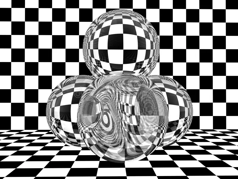
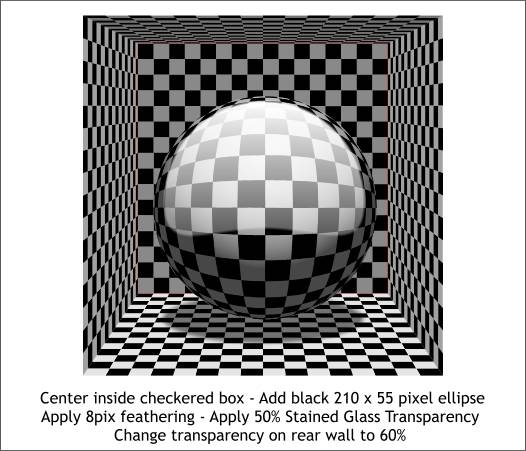
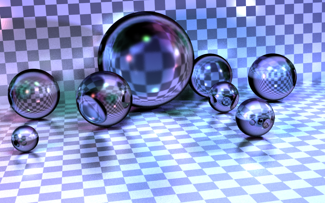
Well, it was time to move on to refraction. There was a huge amount of deliberation getting it to work properly. If you Google for reference images of glass spheres, you'll get things like:
|

|
|
|
Some of these look pretty legit, with caustics and chromatic aberration. I couldn't figure out why my raytracer was giving completely different results. These renders look like the center is shrunk, and even more so at the edges. It should be just the opposite, I thought; the image should be magnified, especially at the edges. I even wrote a 2D case from some ancient code I had lying around:
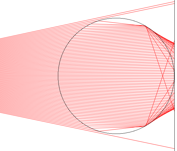
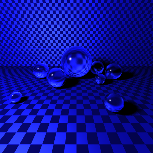
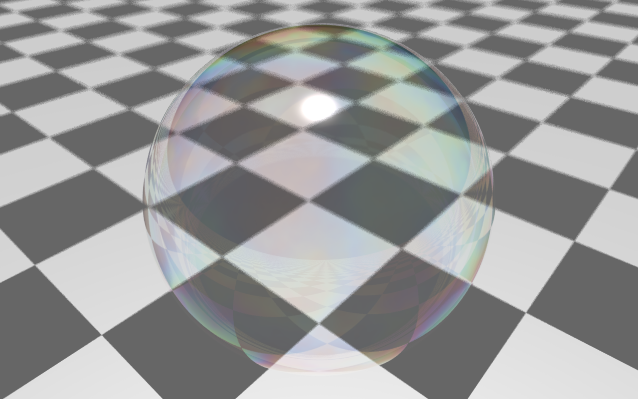
It turns out that the reason the reference images don't match is because they're ALL WRONG. To prove this, I borrowed a marble from Hans Engvall, drew a checkerboard with pencil, and held it up to the light. 'Lo and behold, when the marble is right up against it, the checkerboard is magnified, even more so at the edges! The reference images above can result when you stick a glass sphere a distance from a background—but if it's just sitting up against it, it's dead wrong.
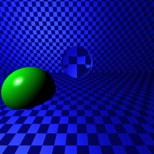
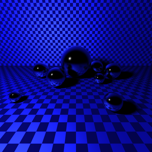
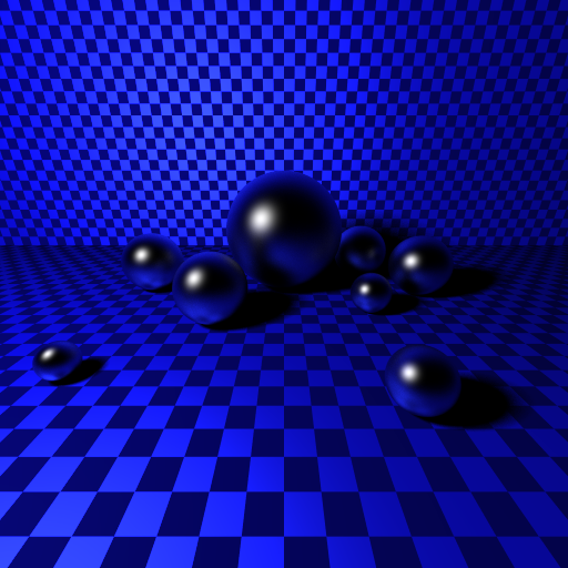
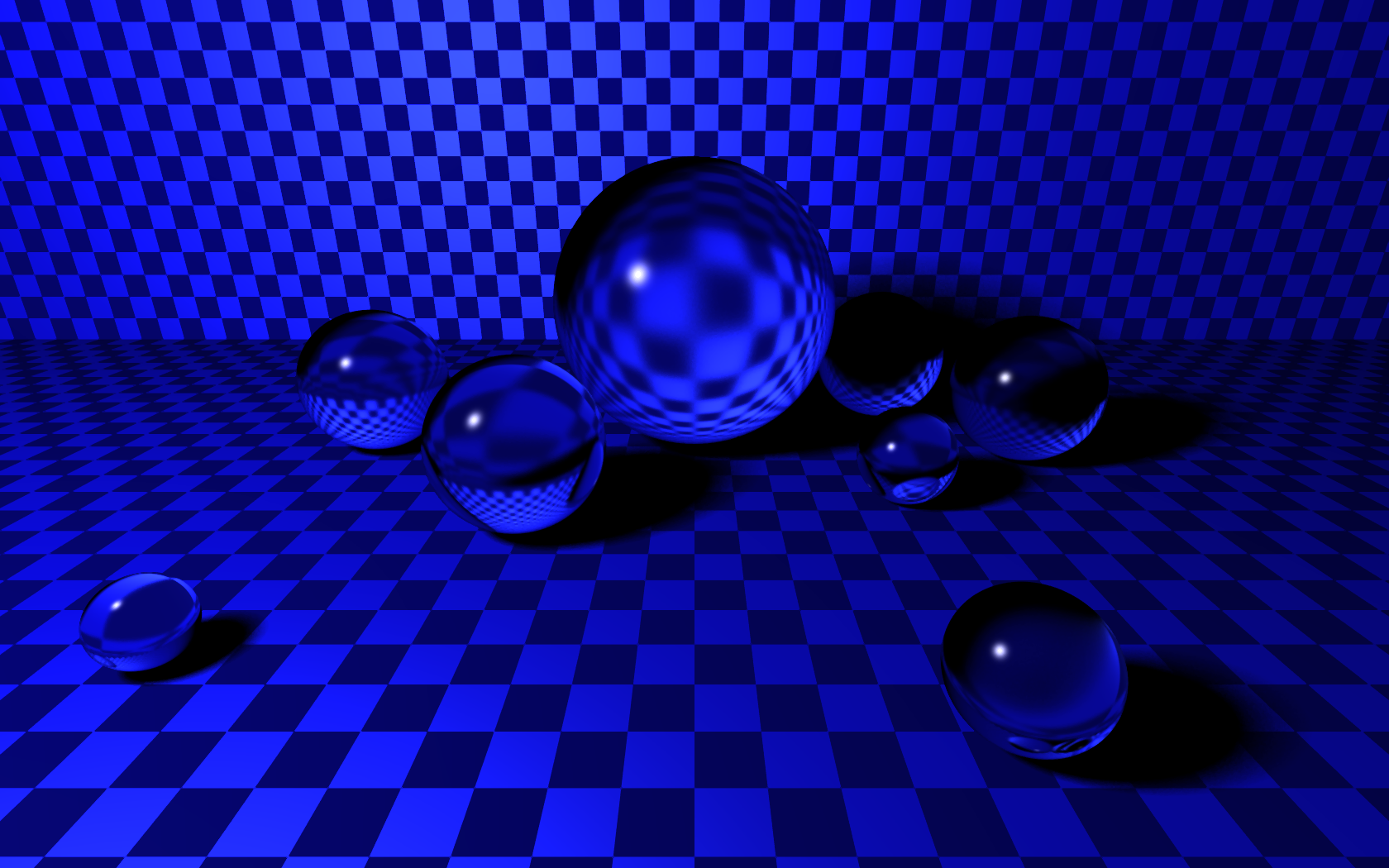
Well, now that that's all sorted out, rendering time! I made a checkerboard hack to all planes (I'll make it real eventually). Bottom-far-left, 100 samples per pixel, 0 reflection samples, 1 refraction sample, 10 shadow samples, in ~53 seconds. Bottom-left, 100 samples per pixel, 0 reflection samples, 1 refraction sample, 0 shadow samples, in ~10 seconds. Bottom-center, 10 samples per pixel, 0 reflection samples, 1 refraction sample, 10 shadow samples, in ~29 seconds (1 thread); notice that the plane is farther away, so the refraction is different.
For good measure, the bottom-center scene was rendered with glossy reflectance. Bottom-right: 50 samples per pixel, 20 reflection samples (specular 100), 0 refraction samples, 10 shadow samples, in 5 minutes, 37½ seconds. Bottom-far-right: 50 samples per pixel, 20 reflection samples (specular 10), 0 refraction samples, 10 shadow samples, in 5 minutes, 53 seconds.
|
|
|
|
|
At this point, I was having some problems, but they seemed to have resolved themselves (perhaps the error occurs when surfaces intersect?). Glossy refractions came pretty easily after glossy reflections, and so the following image was rendered in 4 minutes, 58 seconds.
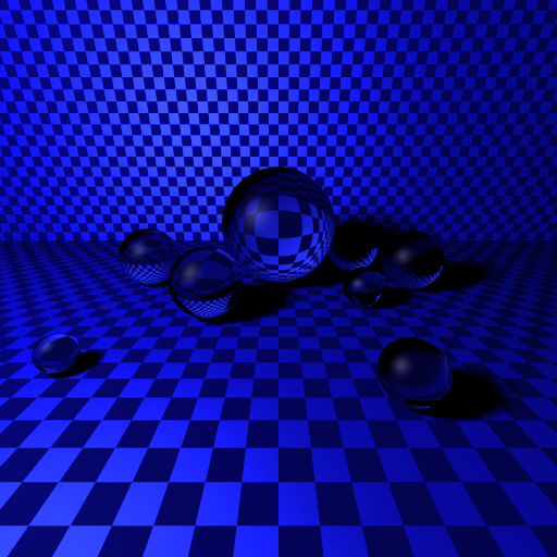
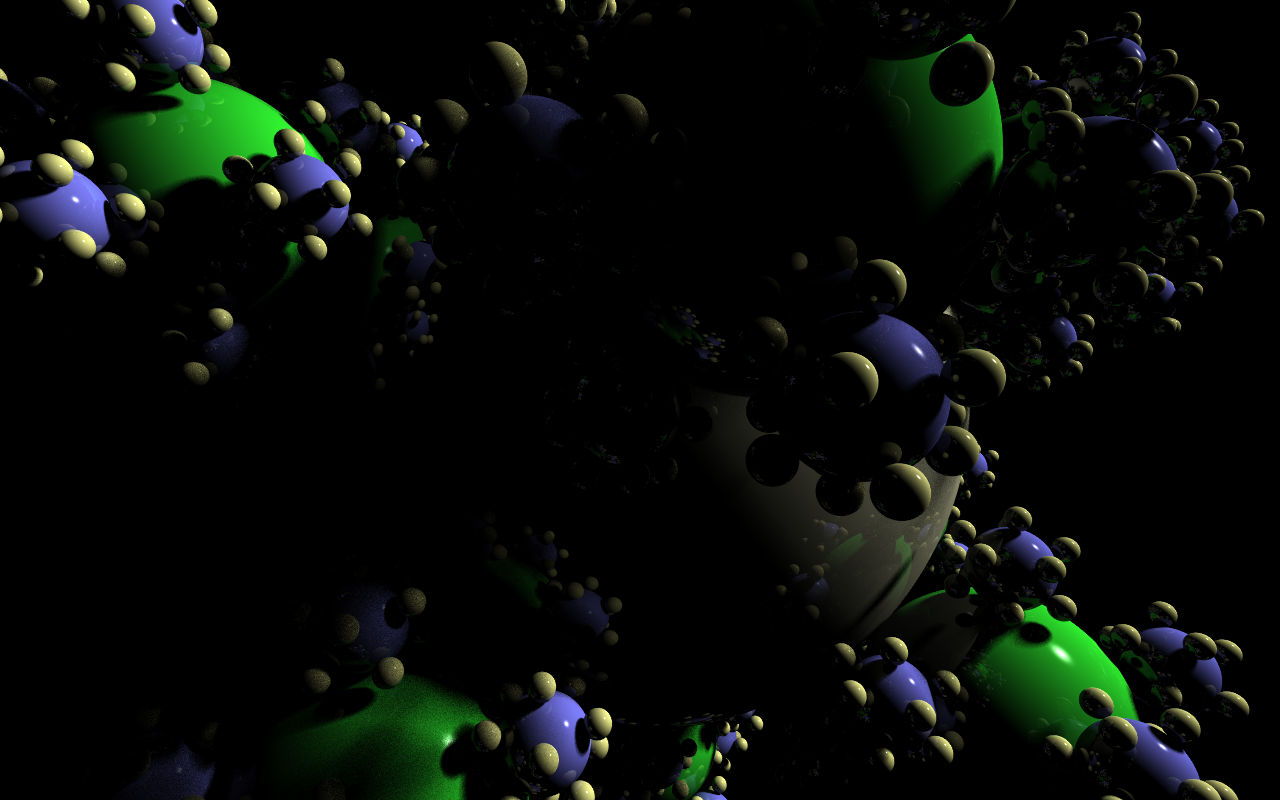
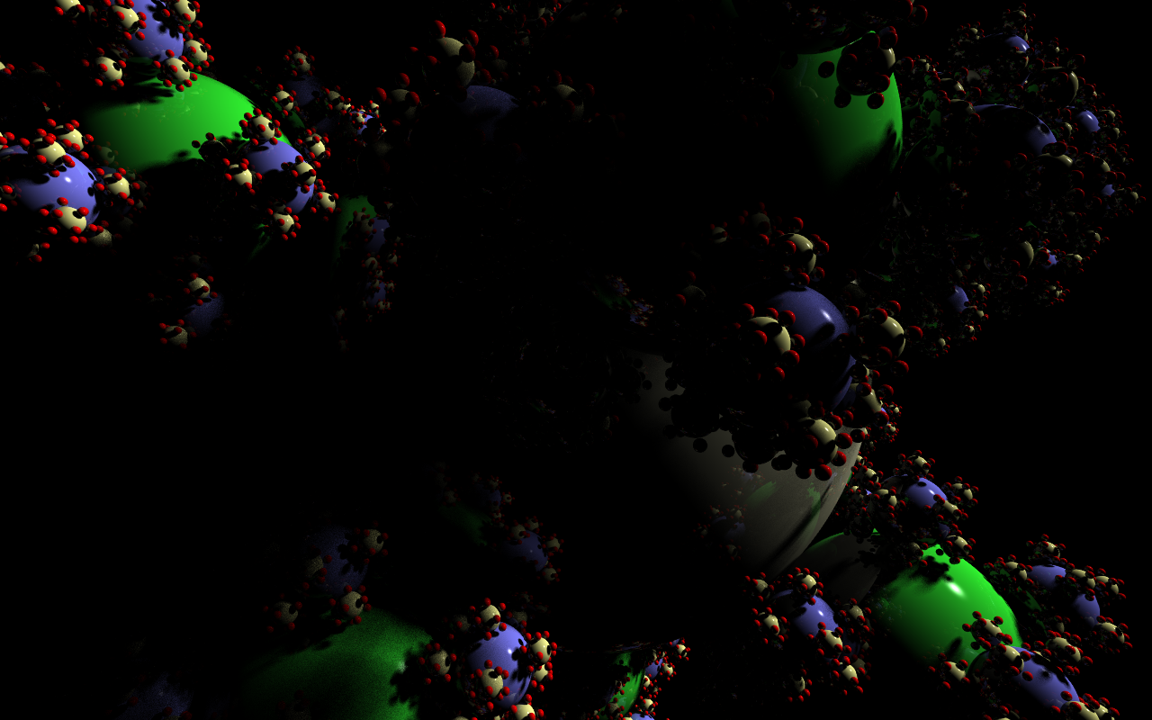
I needed a new desktop background, so I wrote a script that generates a scenefile for my ray tracer. The scenefile is of an icosahedral sphereflake. The image below-left (1280x800, 10 samples/pixel, 1 reflect sample, 10 shadow samples) rendered in 54 minutes, 25 seconds (1597 primitives).
Frankly, this was too slow. I also wanted to do nice things like blurry reflection, more highly sampled shadows, and more depth on the fractal, but the time simply was waaaay too long. I wrote a BVH class of my own design. The BVH is constructed by subdividing a root axis-aligned bounding box into two axis-aligned bounding boxes, the sum of whose volumes is minimal. This data structure would produce the same image an estimated 53.4% faster, based on a small-scale test. To get an idea of how many object tests we're saving, I wrote a counter, that counts how many times the ray was tested. Using this, and several hours of debugging later, I found that my data structure was actually not working (well). I fixed it up by simply choosing the best median of the data when sorted along a cardinal axis, and the same scene rendered in 4 minutes, 26-54 seconds, a speedup of about 12x! I wrote an image diff application, that shows the difference between the two images. The difference is insignificant (and almost humanly invisible), and is entirely due to the fact that random samples were used. Below-right is a visualization of how many tests were done for each pixel (first bounce) for the scene: blue is 0 tests (close to the minimum), bright red is 15 tests (close to the maximum); the maximum bounding volume hierarchy depth was 16; rendered with 10 pixel samples in 4.5 seconds.
|
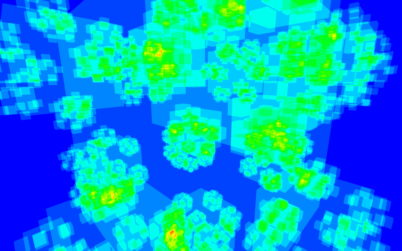
|
Below-right is the next level of the fractal (17,569 primitives), (15 minutes, 35 seconds), and below far-right is the intersection visualization (58½ seconds, same 0 to 15 test scale):
|
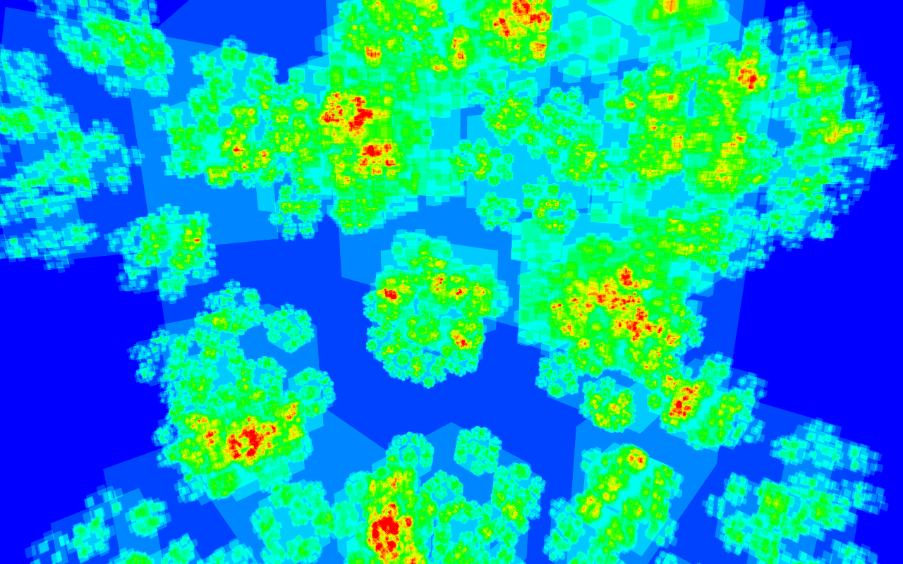
|
Next was to make the shadows softer. With the faster data structure, it was now feasible to use 100 shadow samples. I left the render going and went to class, and then to lunch. The result, in 1 hour, 31 minutes, 16½ seconds:

Very pretty. Now, it was time to fix the samples with something a bit more professional.
Poisson Disk Sampling:
The stochastic supersampling served the ray tracer well, but it was time to kiss it goodbye. The problem with random sampling is that points can cluster (see image, below-left). This is sad, because that's wasted work. Worse, it is conceivable that some parts of a pixel could be completely not sampled, and the result would be utterly wrong. An excellent solution is to use Poisson Disk sampling, which computes sample positions that are roughly equidistant. Poisson Disk sampling is at the bottom-right. Notice how no two samples are close together nor too far apart.
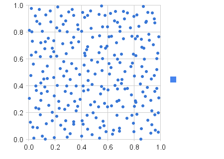
|

|
Great, so let's use Poisson Disk sampling. Turns out that generating those samples is really freaking annoying. At HPG 2011, I saw a paper that describes a nice way to do it on a finite number of points, but it requires lots of work. Because I only gave myself a few hours to do this, Delaunay triangulation was out of the question. Possibly the easiest (while still not outright stupid) method is an elegantly simple algorithm proposed in this paper. Although concise in itself, a decent explanation and, helpfully, implementations, can be found here.
There's a problem with this algorithm, however. It doesn't produce a distribution with an exact number of points. This is problematic. Fortunately, I was clever enough to figure out that you can generate more than that number of samples, and then cut out parts of the domain until you're down to the right number. Then, you can scale that domain up. For example, if you want 100 samples, you can generate 113 samples on a unit square. Then, you can cut out a smaller piece of that square (say, [0 to 0.95]), such that there are exactly 100 samples in that subsquare. You then throw out the other samples, and scale that square back up to the unit square.
It turns out that figuring out a minimum radius (the major control one has over this algorithm's output) that produces just a little bit over the number of samples you need is really hard. Because no one knew how to do this, I derived a hackish solution myself. Given a triangular grid (densest packing), for a distance between points "r", the average point density is 2*(r230.5)-1, which can be derived through basic geometry. You then solve num_points=density*area, where density is the formula before, area is 1.0 (the unit square), and num_points is how many points you want. The answer is 20.53-0.25num_points-0.5. In practice, however, the Poisson Disk is not a perfectly efficient packing. My hackish solution is to replace the square root (num_points-0.5) by (1.25*num_points0.51)-1. In practice, this works well for values between 1 and 30,000, inclusive, which was as far as I tested.
Scaling back up was annoying. In turns out that there isn't a nice way to do this. In practice, I scaled the points such that the lowest point and the highest point touched the edges of the unit square. Then, I scaled it so that 1/4*r was on each side. I used a program I had earlier to determine this (originally, I tried 1/2*r, but it turns out that that's not as nice).
Plugging it back into the renderer, the results improved dramatically. The same results could be achieved with 10 samples that it had previously taken 100 samples (subjectively, anyway; I was too tired to do any real tests).
Here are the Poisson Disk results for a square domain and a circular one (needed for aperture sampling for depth of field; see below) with 2,000 points each.

|
|
At this point, I found a problem with the BVH, which I corrected (I discovered the problem because triangles didn't render). It was time for another render, so in about 34 minutes:
I fixed a bug concerning the lighting (light color wasn't being factored in). I then decided that the above image was somewhat boring, so I changed the scenefile a lot, including setting up three lights and changing the camera. Scenefile:
image {
    width 1280
    height 800
    samples 10
}

camera {
    position 1.5 10 2 center -0.3 0.0 0.1
    up -0.05 0.0 1.0
    image_plane 3.0
}

light "light1" {
    color 1.0 0.5 0.5
    object:sphere { radius 0.5
        position 4 4 2
    }
}
light "light2" {
    color 0.8 0.8 1.0
    object:sphere { radius 0.1
        position -4 2 2
    }
}
light "light3" {
    color 0.5 1.0 0.5
    object:sphere { radius 1.5
        position 0.3 4 6
    }
}

material "plane_material" {
    action:reflect 1.0 2
    action:shadow "light1" 10
    action:shadow "light2" 10
    action:shadow "light3" 10
    diffuse 0.375 0.375 0.75
    specular 1.0 1.0 1.0
    shininess 300
}
material  "sphere1_material" {
    action:refract 1.0 2
    action:shadow "light1" 10
    action:shadow "light2" 10
    action:shadow "light3" 10
    diffuse 0.0 0.0 0.0
    specular 1.0 1.0 1.0
    index 2.414 8000.0
    shininess 100
}

scene {
    background 64 64 64

    object:sphere {
        use "sphere1_material"
        position 0 0 1
        radius 1
    }

    object:sphere { use "sphere1_material" radius 0.5
        position 2.3 0.2 0.5
    }
    object:sphere { use "sphere1_material" radius 0.5
        position 1 1.4 0.5
    }
    object:sphere { use "sphere1_material" radius 0.5
        position -1.5 -0.5 0.5
    }
    object:sphere { use "sphere1_material" radius 0.5
        //position -2.3 0.4 0.5
        position -2.6 0.4 0.5
    }
    object:sphere { use "sphere1_material" radius 0.3
        position -1.3 1.1 0.3
    }
    object:sphere { use "sphere1_material" radius 0.3
        position -1.2 3.0 0.3
    }
    object:sphere { use "sphere1_material" radius 0.2
        position 2.3 2.6 0.2
    }

    object:plane {
        use "plane_material"
        position 0 0 0
        normal 0 0 1
    }
    object:plane {
        use "plane_material"
        position 0 -1.5 0
        normal 0 1 0
    }
}
This results in:
So far, so good. I still needed depth of field. Depth of field is based off of an actual camera model; because my camera model assumed that image plane was in front of the center of projection, I had to make some changes. I put the image plane behind the center of projection, and sent the rays through the center of projection.
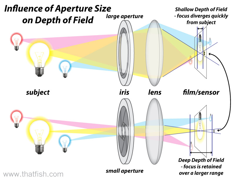
To add depth of field, one jitters the center of projection to simulate a lens. I used the thin lens approximation and some basic Geometry to derive the necessary "refraction": all we care about is the focal point, so that is calculated first from the image plane location. After this, all that need happen is for random points on the lens to be shot through the focal point. The aperture and the lens are assumed to be one unit. A lens is circular, so I added code to my Poisson Disk implementation to allow it to generate random points inside a circular domain (see pictures in the subsection above). In practice, using the same sampling pattern for each pixel (or subpixel) sample leads to aliasing. I corrected this by using 50 sampling patterns, and then randomly selecting one for each sample.
Thus, if an object is at the focal point, all rays from the point on the image plane through the lens to that object will be in focus. If an object is before or behind that focal point, those rays diverge, making the object blurry. I found the following image helpful:
The first (correct) depth of field image, with aperture 0.1 (10 aperture samples) and focal length 0.75, 1 reflection sample on the triangle, 1 shadow sample, and 10 samples per pixel in 10½ seconds:
Some tweaks and:
 Version 4:
Version 4 adds .obj file loading support, texturing support, and some bug fixes. I'll be honest, there's actually more bugs than when I started. This may be due in large part to the fact that I thought it would be neat to fail to attempt to rewrite the scene parser. The resultant code is actually not bad, but it's not fully functioning yet.
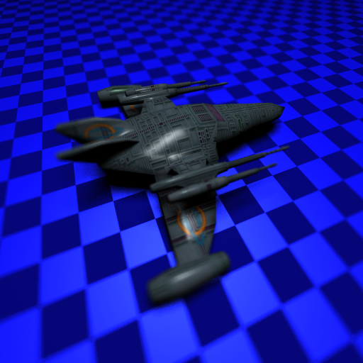
The texturing works with nearest, bilinear, bicubic, and Gaussian (normal) filtering modes[4]. A comparison is below (note the heavy blurring on the Gaussian filter):
|

|

|

|
| 52.27 seconds | 49.09 seconds | 56.67 seconds | 28.38 seconds (incorrect?) |
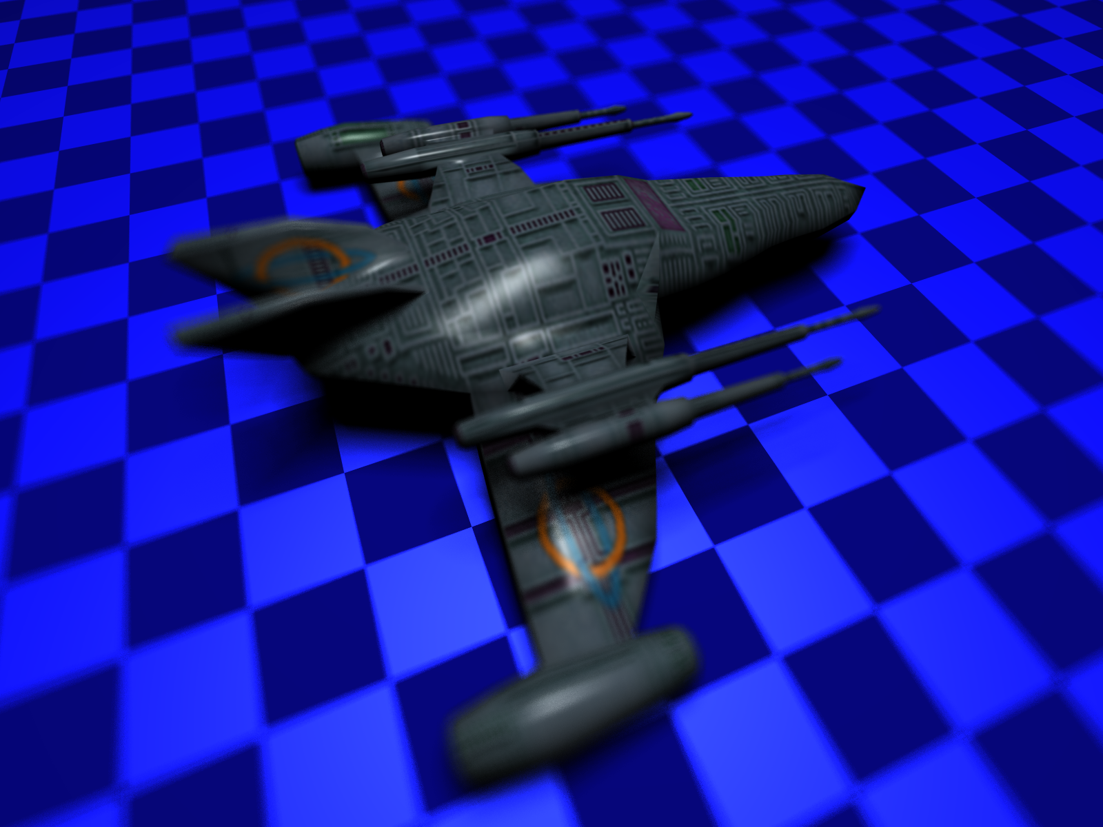
The tests were rendered from the following scenefile of a little toy spaceship:
image {
    width 512
    height 512
    samples 100
}

camera {
    position 1.0 1.0 0.5 center 0.0 -0.7 0.1 up 0.0 1.0 0.0
    image_plane 1.0
    aperture 0.1 2
    focal 0.55
}

light "light1" {
    color 1.0 1.0 1.0
    object:sphere {
        radius 1.0
        position 0 4 0
    }
}

material "plane_material" {
    action:refract 0.2 1
    action:shadow "light1" 1
    diffuse 0.05 0.05 1.0
    specular 0.2 0.3 1.0
    shininess 3
}

scene {
    background 64 64 64

    object:plane {
        use "plane_material"
        position 0 -0.22645799815654755 0
        normal 0 1 0
    }
    object:obj {
        model "data/Spaceship.obj"
        //position 0.0 0.0 0.0
    }
}
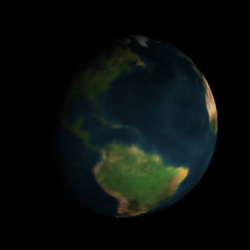
The following test uses a texture (deliberately downsized to better show aliasing) on a raytracing primitive (i.e., a sphere). The effect of space has been crudely simulated by removing specular and changing the background color to black.

|
|

|

|
| 7.52 seconds | 9.63 seconds | 14.84 seconds | 5.18 seconds (incorrect?) |
The tests were rendered from the following scenefile (of the Earth, I hope you know):
image {
    width 512
    height 512
    samples 100
}

camera {
    position 1.0 -1.0 -1.5 center 0.0 0.0 1.0 up 0.0 -1.0 0.0
    image_plane 2.0
}

light "light1" {
    color 1.0 1.0 1.0
    object:sphere {
        radius 1.0
        position 6 0 -2
    }
}

material "plane_material" {
    action:refract 0.2 1
    action:shadow "light1" 1
    diffuse 0.05 0.05 1.0
    specular 0.2 0.3 1.0
    shininess 3
}
material  "sphere1_material" {
    action:shadow "light1" 2
    diffuse 1.0 1.0 1.0

    //https://atmire.com/labs17/bitstream/handle/123456789/7618/earth-map-huge.jpg?sequence=1
    texture_diffuse "data/earth.png"

    specular 0.0 0.0 0.0
    shininess 1
}

scene {
    background 0 0 0

    object:sphere {
        use "sphere1_material"
        position 0 0 1
        radius 1
    }
}
The source distribution includes the resources needed to create and use these scenefiles.
Version 5:
Version 5 adds bug fixes, and Beer's Law. Mostly, I've been working on OptiX and final projects, so the code's fairly incremental and not-robust. The CPU ray tracer is being rewritten into a path tracer also.
 Version 6:
Version 6 improves a lot.
The architecture of the underlying library has been changed dramatically. The OpenGL basecode was completely refactored to use namespaces. In addition, the library is now const-correct! Given the scope of the library, this was a substantial undertaking. In addition, the library itself was generally cleaned up in a few places.
The ray tracer was also significantly revamped. I fixed a semantic error in the refraction function, and changed stuff around to compensate. The functions' rudimentary return values have been swapped out for returning structs of data, and they now take ray arguments. This had the immediate effect of making everything a lot more readable, but it can also be justified from a performance perspective, as the objects now allow values to be cached.
I changed the semantics of how the Beer–Lambert law is calculated, and added Fresnel coefficients.
I also got some path tracer code from the internet in preparation for making a bi-directional path tracer.
I looked into a problem I've been having with the refraction. I first noticed the problem a while ago; sometimes vectors will try to pop the material stack, but it will fail because it's already empty. As it turns out, there are three (root) causes: 1, that I was handling total internal reflection incorrectly, 2, that the offset epsilon for a vector pushes the vector through another surface, and 3, that smoothed geometry normals can screw things up. There's not much I can do about the second one, so for now I'm just outputting an error color. As for the third, I don't have a satisfactory solution, other than to not use smoothed geometry. I'm thinking maybe a subpixel triangulation step à la the REYES architecture. Obviously, in this release, the first is fixed.
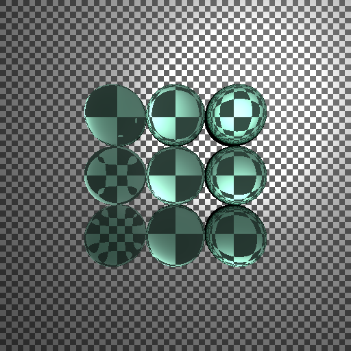
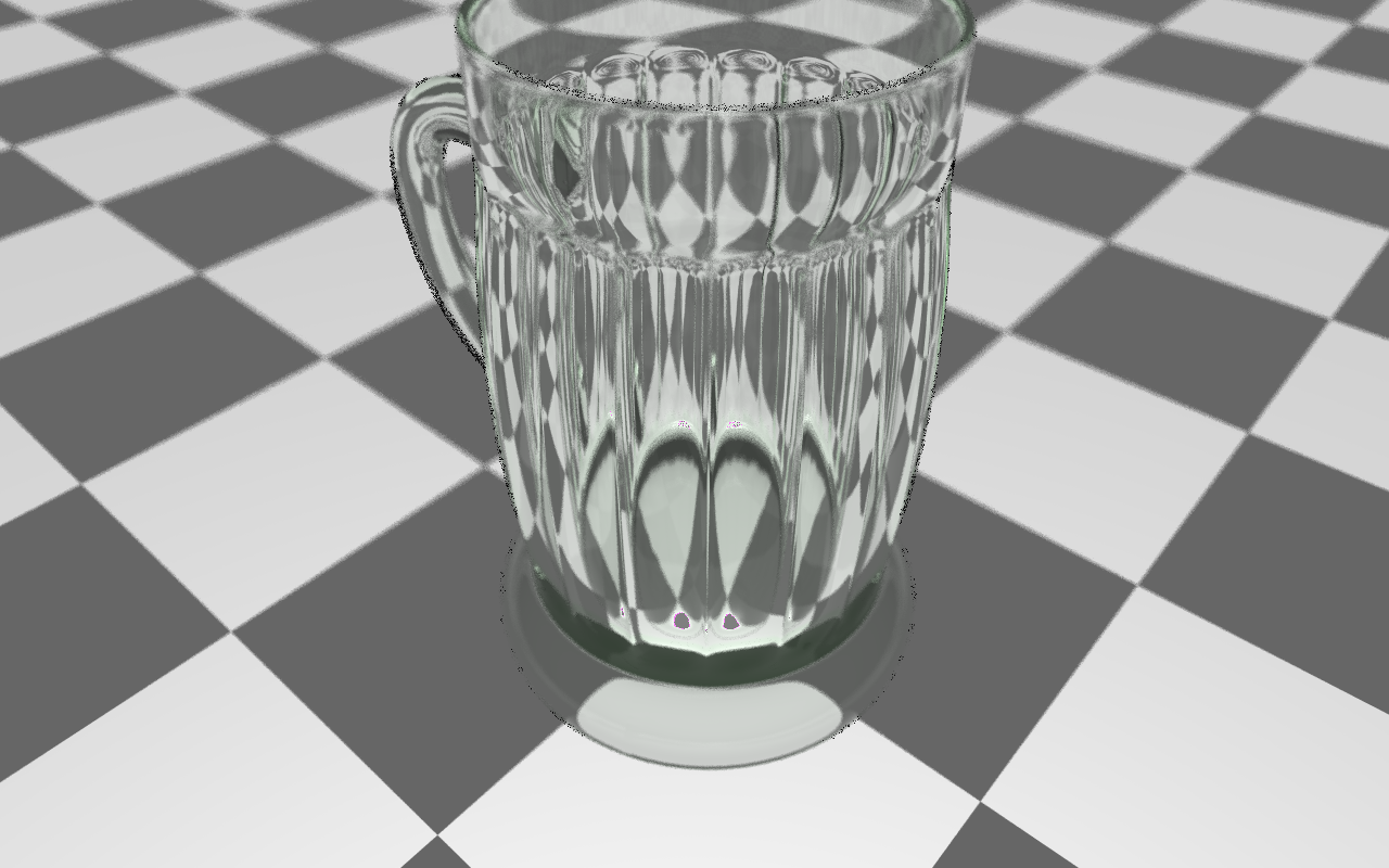
The path tracer is sorely needed. Almost all of the time spent rendering the images below was in the glass. There is a maximum recursion depth of 4 in both images, and a reflection ray and refraction ray are calculated for (most of) them. This leads to 24=16 rays. Originally, I had a maximum depth of 16 . . .
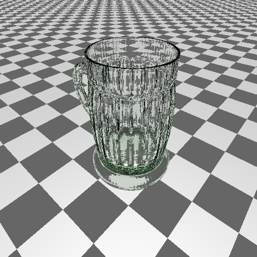 ~51 seconds
 Version 7:
Version 7 refactors the code significantly, fixing many bugs, and simplifying code immensely. Functionally speaking, there were two main additions: thin film interaction, and the path tracer!
In this section, please note that times may be somewhat inaccurate or misleading, because the conditions were not carefully controlled, and many changes were made in-between images.
Thin film was surprisingly difficult to get right. In the end, it isn't quite right (although it is physically based). The basic idea of thin film interaction is that light reflects off of two surfaces. Basically, the waves of light interfere constructively or destructively. The following diagram explains:
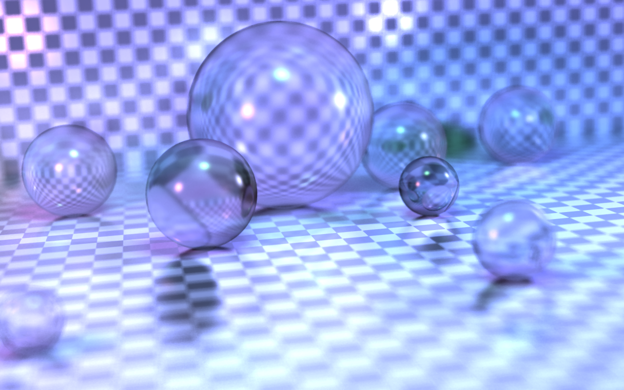
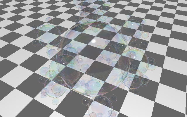
My model does not take into account distance AD, nor the 180° phase shifts associated with interacting with the medium itself. However, the following images of soap bubbles are fairly compelling (uses a Perlin noise implementation, in the public domain, to perturb the film thickness).
Path Tracing:
I found some helpful code that gave me an excellent starting point. After deobfuscating, cleaning up, and improving the code, I rewrote it using my library into the ray tracer. There is a #define that allows one to quickly switch back and forth between path tracing and Whitted ray tracing as render methods.
The following image is my first (reasonably successful) path tracing image (renders very quickly):
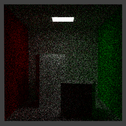
This image is wrong—and I knew that at the time it was rendered. The distribution used for diffuse in this image was an unweighted hemispheric distribution. I already had a library function for this (glLib::Math::Random::get_hemisphere(...)) which can be overloaded to take a vector (normal) to define the center of the hemisphere. Unfortunately, Lambertian surfaces should be cosine weighted (probability of going sideways is zero, high probability of going close the normal).
The uniform random hemisphere is a straightforward random distribution to generate: simply generate a random point on the surface of a unit sphere (normalize three Gaussian samples) and then flip points about the plane defined by the normal and the origin, if necessary. I also had a cosine weighted hemisphere sample, but it was restricted to (effectively) a normal pointing along one axis. The way this works is that a random point is generated on a flat disk (uniformly choose an angle, and then let radius be the square root of a uniform variable), and then that 2D point is projected up to the surface of the hemisphere (z = sqrt(1-x*x-y*y), by the Pythagorean Theorem).
To make a cosine weighted distribution that could have a variable normal, some Linear Algebra must be applied. After some false starts, I figured it out with a hint from a presentation: simply construct an (any) orthonormal basis {X,Y,N} (the normal is the third), scale vectors X and Y by the x and y points of the disk sample, scale N by z, and then add it all up. Effectively, this just does a change of basis from {i,k,j} to {X,Y,N}. Because the distribution is rotationally symmetric about N, we don't care what X and Y are, so long as they form an orthonormal set with N. In practice, X can be easily found by applying the cross product to N and a different vector (one of i, j, xor k, depending on which is least like N). Once X is normalized, Y may be found as the cross product of N and X (note that because N and X are orthonormal, Y does not need to be normalized).
With the cosine weighting:
Some improvements later, and it was time to render a large image. With the scenefile (based, loosely, on the Cornell Box data):
image {
    width 1024
    height 1024
    samples 1000
}

camera {
    position 278 273 -800 center 278 273 -799 up 0.0 1.0 0.0
    image_plane 2.7
    aperture 0.1 1
    focal 0.035
}

material "light" {
    emission 12.0 12.0 12.0
    shininess 3
}
material "white" {
    diffuse 1.0 1.0 1.0
    shininess 3
}
material "red" {
    diffuse 1.0 0.0 0.0
    shininess 3
}
material "green" {
    diffuse 0.0 1.0 0.0
    shininess 3
}

scene {
    background 64 64 64

    //Light
    object:triangle {
        use "light"
        position  343.0 548.5 227.0
        position2 343.0 548.5 332.0
        position3 213.0 548.5 332.0
    }
    object:triangle {
        use "light"
        position  343.0 548.5 227.0
        position2 213.0 548.5 332.0
        position3 213.0 548.5 227.0
    }

    //Floor
    object:triangle {
        use "white"
        position  552.8 0.0   0.0
        position2   0.0 0.0   0.0
        position3   0.0 0.0 559.2
    }
    object:triangle {
        use "white"
        position  552.8 0.0   0.0
        position2   0.0 0.0 559.2
        position3 549.6 0.0 559.2
    }

    //Ceiling
    object:triangle {
        use "white"
        position  556.0 548.8   0.0
        position2 556.0 548.8 559.2
        position3   0.0 548.8 559.2
    }
    object:triangle {
        use "white"
        position  556.0 548.8   0.0
        position2   0.0 548.8 559.2
        position3   0.0 548.8   0.0
    }

    //Back wall
    object:triangle {
        use "white"
        position  549.6   0.0 559.2
        position2   0.0   0.0 559.2
        position3   0.0 548.8 559.2
    }
    object:triangle {
        use "white"
        position  549.6   0.0 559.2
        position2   0.0 548.8 559.2
        position3 556.0 548.8 559.2
    }

    //Left wall
    object:triangle {
        use "red"
        position  552.8   0.0   0.0
        position2 549.6   0.0 559.2
        position3 556.0 548.8 559.2
    }
    object:triangle {
        use "red"
        position  552.8   0.0   0.0
        position2 556.0 548.8 559.2
        position3 556.0 548.8   0.0
    }

    //Right wall
    object:triangle {
        use "green"
        position  0.0   0.0 559.2
        position2 0.0   0.0   0.0
        position3 0.0 548.8   0.0
    }
    object:triangle {
        use "green"
        position  0.0   0.0 559.2
        position2 0.0 548.8   0.0
        position3 0.0 548.8 559.2
    }

    //Short block
    object:triangle {    use "white"    position  130.0 165.0  65.0     position2  82.0 165.0 225.0    position3 240.0 165.0 272.0}
    object:triangle {    use "white"    position  130.0 165.0  65.0     position2 240.0 165.0 272.0    position3 290.0 165.0 114.0}
    object:triangle {    use "white"    position  290.0   0.0 114.0    position2 290.0 165.0 114.0    position3 240.0 165.0 272.0}
    object:triangle {	use "white"	position  290.0   0.0 114.0	position2 240.0 165.0 272.0	position3 240.0   0.0 272.0}
    object:triangle {	use "white"	position  130.0   0.0  65.0	position2 130.0 165.0  65.0	position3 290.0 165.0 114.0}
    object:triangle {	use "white"	position  130.0   0.0  65.0	position2 290.0 165.0 114.0	position3 290.0   0.0 114.0}
    object:triangle {	use "white"	position   82.0   0.0 225.0	position2  82.0 165.0 225.0	position3 130.0 165.0  65.0}
    object:triangle {	use "white"	position   82.0   0.0 225.0	position2 130.0 165.0  65.0	position3 130.0   0.0  65.0}
    object:triangle {	use "white"	position  240.0   0.0 272.0	position2 240.0 165.0 272.0	position3  82.0 165.0 225.0}
    object:triangle {	use "white"	position  240.0   0.0 272.0	position2  82.0 165.0 225.0	position3  82.0   0.0 225.0}

    //Tall Block
    object:triangle {	use "white"	position  423.0 330.0 247.0	position2 265.0 330.0 296.0	position3 314.0 330.0 456.0}
    object:triangle {	use "white"	position  423.0 330.0 247.0	position2 314.0 330.0 456.0	position3 472.0 330.0 406.0}
    object:triangle {	use "white"	position  423.0   0.0 247.0	position2 423.0 330.0 247.0	position3 472.0 330.0 406.0}
    object:triangle {	use "white"	position  423.0   0.0 247.0	position2 472.0 330.0 406.0	position3 472.0   0.0 406.0}
    object:triangle {	use "white"	position  472.0   0.0 406.0	position2 472.0 330.0 406.0	position3 314.0 330.0 456.0}
    object:triangle {	use "white"	position  472.0   0.0 406.0	position2 314.0 330.0 456.0	position3 314.0   0.0 456.0}
    object:triangle {	use "white"	position  314.0   0.0 456.0	position2 314.0 330.0 456.0	position3 265.0 330.0 296.0}
    object:triangle {	use "white"	position  314.0   0.0 456.0	position2 265.0 330.0 296.0	position3 265.0   0.0 296.0}
    object:triangle {	use "white"	position  265.0   0.0 296.0	position2 265.0 330.0 296.0	position3 423.0 330.0 247.0}
    object:triangle {	use "white"	position  265.0   0.0 296.0	position2 423.0 330.0 247.0	position3 423.0   0.0 247.0}
}
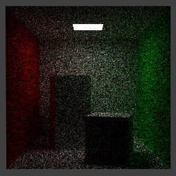
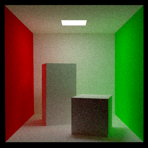
The following 1024x1024 image has 1000 samples per pixel, and took 1 hour, 34 minutes, 10 seconds (on the Linux machines in the UNM computer lab):
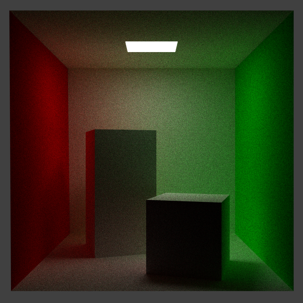
Okay, pretty noisy, but a good result! I remember hearing that convergence of Monte Carlo methods is with the square root of n. So, we'd need 4000 samples to make it twice as good. Denoised:
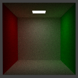
It looked to me like there might be too much color bleeding (radiosity). 256x256 test image with no boxes with 4000 samples per pixel, and denoised, in 24 minutes, 37 seconds:
|
|
Notice the soft shadows the area light source casts, as well as the radiometric effects (color bleeding). I'm not certain everything is entirely correct, but it's definitely a great start.
If this the final post on this project, it's certainly not the end. I have always wanted to do graphics, and despite everything I've done, I've still only just gotten my feet wet.
Happy tracing!
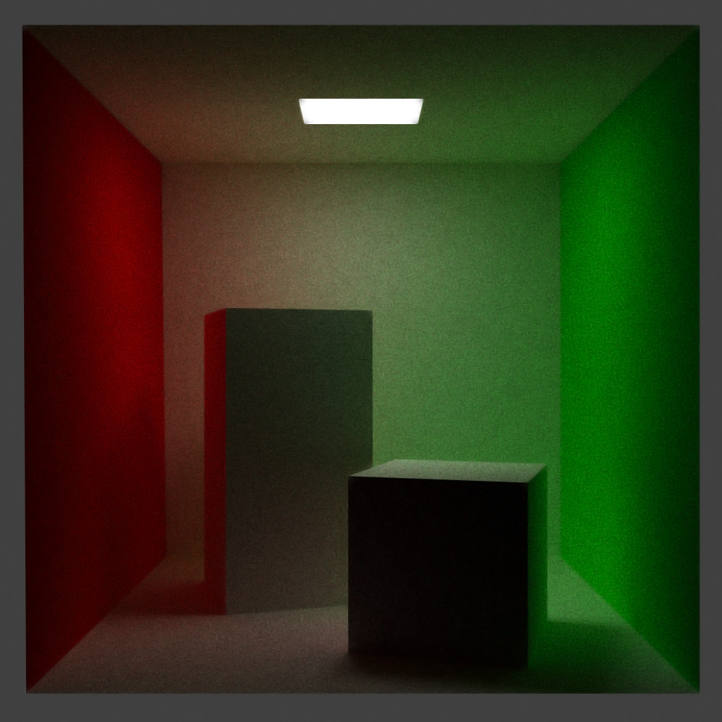
Update: the final project for this class consisted of three images, presented below. All used 1,000 samples per pixel, and took about an hour to render, some on my computer and some on the CS machines. The code change required for reflection and refraction was comparatively minor and is not currently available for download. The extra radiosity issue appears to just be an issue with tonemapping—so it's not an issue.
|
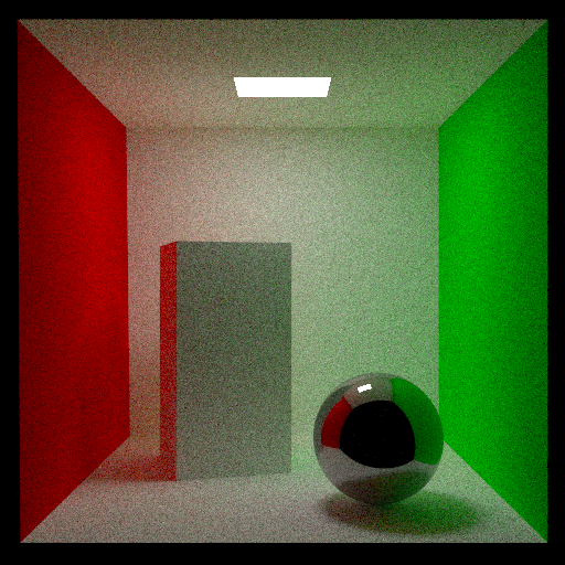
|
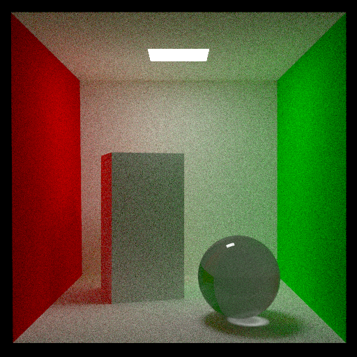
|
Source:
Version 1:
Currently standalone (though does require SDL and STL), but I hope to eventually integrate it into the (less advanced but more robust, clean, and flexible) ray tracer in glLibC, my C++ graphics library.
Version 2:
Some speed issues on Linux. All the fancy features described in Version 1.
Version 3:
Still the speed issues on Linux? All the fancy features described in Version 2.
Version 4:
Still the speed issues on Linux (but hey, it compiles!)? All the fancy features described in Version 3.
Version 5:
Version 6:
Version 7:
Runs on Linux, too!
Thanks for reading!
-Agatha Mallett
[1]Technically, there was other stuff too. I removed the comments and some unused data. This is the important part, anyway.
[2]CPU: Intel Core 2 Duo (2.4GHz, two cores)
[3]The ray tracer optimizes the reflection sample count of 1 to be mirror reflection. Perhaps this isn't a good idea. Anyway, it meant that to test distributed glossy reflection, the sample count had to be 2.
[4]The Gaussian filter uses the standard normal distribution with a standard deviation equal to one pixel's span. By default, the filter extends four standard deviations (a total of 64 samples).
Page last substantively updated 2011-10-03. Maintenance and minor updates were applied later.