Light and Color: Introduction to Radiometry, Photometry, and Colorimetry
Introduction
Radiometry, Photometry, and Colorimetry are in some sense pre-requisites to rendering, but they are not rendering per-se.
Put simply, Radiometry (literally: "light measurement") is the science of how light works—the actual physical photons moving around the world. When we are writing a renderer, we are simulating this actual
Conversely, Colorimetry is the perceptual study of how light appears to the human visual system. There's quite a bit of science in it, too. Colorimetry depends upon the light simulated from Radiometry. It is the final step in rendering, not the tool to render per-se.
Photometry blends the two, doing light measurement weighted by human luminance sensitivity. Photometry is mainly useful for people who are not doing graphics, but it is frequently confused with Radiometry, and comes with its own units that we do need to deal with when creating rendered images for display.
Radiometry and Radiometric Units
Radiometry describes how actual light propagates. In graphics, it is the tool that lets us figure out how much light from the light source(s) in the scene is absorbed by sensor(s) of the scene (think: cameras or eyes). Taking pathtracing as an example, we randomly select paths from the sensor(s) to light source(s). Estimating the light propagating along the path, and averaging the results of many such estimates in the careful formalism of a Monte Carlo method, gives us the total light hitting the pixel.
Understanding Radiometry, separate from a rendering technique, is mostly a question of understanding what the units are. We'll define all units below, but to give a flavor: the light from the light sources is usually measured in
Radiometry works in physical units, based on SI[1]. Unfortunately, the units have a rich history and their names are sometimes used for different things in other fields (mainly in Physics). The usage here will be correct for graphics.
It's important to note that there are also
In graphics, we really 'should' be talking about spectral units, since these are the units in which you actually write your renderer. However, in practice, this is an extra dimension and it's obvious from context anyway which one we're talking about, so most of the time everyone just drops the distinction and describes their renderer in non-spectral units.
Without further ado, everyone who does physically based rendering thoroughly knows and understands the following radiometric quantities:
Radiant Energy
Radiant Flux
You usually only see radiant flux by itself at the beginning or end of rendering (the power of the lights or the power accumulated on the sensor, respectively). However, throughout the rendering process, other quantities are used, all based on radiant flux as a primitive.
The units of radiant flux are Watts (\(\unitsW\)), and the ubiquitous symbol is \(\Phi\).
Radiant Flux Density: Irradiance, Radiant Exitance, Radiosity
The most common place you see irradiance nowadays is in the rendering equation. The incoming radiance (see below) gets multiplied by the geometry term, which converts to differential area on the surface, while we're integrating over the (hemi)sphere, which cancels the differential solid angle—together, the result is irradiance. (Note that the BRDF/BSDF is the ratio of outgoing radiance to incoming radiance, so multiplying by it gives us radiance for the final output, propagating the cycle to the next bounce.)
Radiant Intensity
Radiance, Importance
Radiance is the common intermediary when doing rendering because, amazingly, it is invariant along straight rays (that is, it doesn't change with distance). This makes some sense if you remember the intuitive definition as brightness: a lightbulb doesn't look brighter per-se when you get closer to it. You certainly receive more energy because it fills more of your field of view, but any individual point on it doesn't look brighter. This property of distance invariance makes radiance extremely convenient for rendering.
The units for both radiance and importance are Watts per steradian per projected area (\(\unitsL\)). Importance doesn't have a standard symbol, but the symbol for radiance is[3] \(L\):
\[ L ~~=~~ \frac{ d^2 \Phi }{ d\omega ~dA \cos(\theta) } ~~=~~ \frac{ d^2 \Phi }{ d\omega ~dA^\perp } \]Using \(dA^\perp\) is probably the better notation: it stresses that the differential area is considered to be perpendicular to the direction of the ray. However, the cosine is nice for showing how it can be canceled in the rendering equation.
Photometry
Photometry is like Radiometry, except that it describes perceptual brightness. While Radiometry concerns the physical power of light, Photometry says how it looks. In Radiometry, we might consider a single photon, which has a spectral radiant energy: the joules carried by that particular photon. What Photometry tells us is how much this matters to perception.
SI defines that light at \(540~\unitsTHz\) will produce exactly \(K_{\text{cd}}:=683~\units{\unitlm/\unitW}\) of luminous flux.
What's luminous flux? Basically, it's radiant flux (\(\unitsW\)), but centered around how bright it looks to a human, giving a new unit, the lumen (\(\units{\unitlm}\)). Just like there are radiometric units built around watts, there are photometric units built around the lumen. For example, radiant intensity (radiometric, \(\units{\unitW/\unitsr}\)) corresponds to luminous intensity (photometric, candela \(\units{\unitcd}\)). (For all the correspondences, see table in next section.)
Of course, photons come at many different frequencies, and perceived brightness varies with respect to that. E.g., if the photon is red or violet, it won't look as bright as if it were green. The way we handle this is by a dimensionless weighting function, the luminous efficiency function \(V(\lambda)\), which says how bright a wavelength \(\lambda\) looks to the human eye, expressed relative to the peak value, \(V(555~\unitsnm) = 1\). In practice, \(V(\lambda)\) is tabulated data that you can just download.
The \(540~\unitsTHz\) light above was chosen to have a wavelength close to \(555~\unitsnm\). Still, it's a bit off (\(\lambda \approx 555.016~\unitsnm\)), meaning that light at exactly \(540~\unitsTHz\) is actually a smidge dimmer than the peak[4]. Specifically, \(540~\unitsTHz\) (\(\approx 555.016~\unitsnm\)) light produces \(K_{\text{cd}}:=683~\units{\unitlm/\unitW}\) of luminous flux, while \(555~\unitsnm\) light produces \(K_{\text{cd},\lambda}=683.002~\units{\unitlm/\unitW}\) of luminous flux.
For a combination of different wavelengths, we integrate the spectrum with the weighting function. Formally, for a given spectral power distribution (SPD), computed from Radiometry, of radiant intensity \(I(\lambda)\), we integrate, weighting by \(V(\lambda)\), to get the corresponding photometric quantity, luminous intensity \(I_v\), of the whole spectrum:
\[ I_v = K_{\text{cd},\lambda}\int_0^\infty I(\lambda) \, V(\lambda) \, d\lambda \] \[ K_{\text{cd},\lambda} = 683.002~\units{\unitlm/\unitW} \](Note: it is unclear whether this is supposed to be an integral or a sum per-wavelength. For the CIE standard observer (discussed below), it is definitely sums, and so this related function is probably also a sum.)
Note that this equation works for any corresponding units. Although it is defined for radiant intensity vs. luminous intensity, it will also work for radiance vs. luminance, for radiant flux vs. lumens, and so on.
Photometric units are not yet commonly used in computer graphics because the non-physical-ness seems repellant to accurate simulation of light. However, as we shall see below, we can't get around invoking at least a little bit of Photometry for image display. Outside of graphics, Photometry is very popular in fields such as architecture and consumer lighting, where it allows for rough estimations of indoor illumination.
Radiometric and Photometric Units Summary
| Radiometry | Photometry | |||
|---|---|---|---|---|
| Quantity | SI Unit | Symbolic | Quantity | SI Unit |
| Radiant Energy | \(\unitsJ\) | \(Q\), \(J\) | \(\units{\unitlm\cdot\unitsec} = \units{\unitcd\cdot\unitsr\cdot\unitsec}\) ( | |
| Radiant Flux | \(\unitsW\) | \(\Phi\) | \(\units{\unitlm} = \units{\unitcd\cdot\unitsr}\) ( | |
| Irradiance | \(\unitsE\) | \(E=d\Phi_{\text{in}}/dA\) | \(\units{\unitlx} = \units{\unitlm/\unitm^2} = \units{\unitcd\cdot\unitsr/\unitm^2}\) ( | |
| Radiant Exitance | \(\unitsE\) | \(M=d\Phi_{\text{out}}/dA\) | \(\units{\unitlm/\unitm^2}\) (note[6]) | |
| \(\units{\unitJ/\unitm^2}\) | \(\units{\unitlx\cdot\unitsec}\) | |||
| Radiant Intensity | \(\units{\unitW/\unitsr}\) | \(I=d\Phi/d\omega\) | \(\units{\unitcd} = \units{\unitlm/\unitsr}\) ( | |
| Radiance | \(\unitsL\) | \(L=d^2\Phi/(d\omega\cdot dA^\perp)\) | \(\units{\unitcd/\unitm^2} = \units{\unitlm/(\unitsr\cdot\unitm^2)}\) ( | |
Colorimetry
We have an incoming spectrum of light calculated from Radiometry. If the virtual world were real, that spectrum of light would be real. It would be entering our eyes and giving an impression of color and brightness. The goal of Colorimetry is simply to set pixels on the screen that will induce a similar impression when the viewer looks at it.
A key reference for the details of colorimetric calculations is CIE 015 (older 3rd Ed. for free here or here).
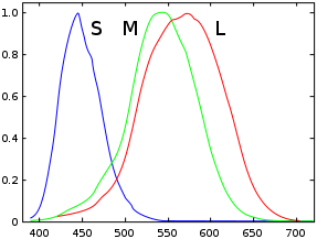
Figure 1
: Approximate standard "long" ("L") / "medium" ("M") / "short" ("S") cone sensitivities as functions of frequency, normalized to \(1.0\). (Image Source)
Cone Response
Most people have three different kinds of color receptors in their eyes (see response functions in Figure 1), which are sensitive to broad, different, ranges of electromagnetic radiation. For example, if \(450~\unitsnm\) light enters your eye, the 'short' cones are stimulated strongly. If \(600~\unitsnm\) light enters your eye, the 'long' cones are stimulated strongly, while the 'medium' cones are stimulated only somewhat. In general, each input produces a response for each of the three types of cone.
Usually, of course, an entire spectral power distribution, comprising many different frequencies at different strengths simultaneously, enters your eye all at once. The cones' response is just the integral of their response over wavelength, and you still only get one response for each type of cone. At the end of the day, it is only these three scalar values that go to your brain to represent that whole infinite-dimensional space of possibility!
Mathematically, for a given spectral power distribution computed from Radiometry, which describes the relative strength[7] of radiation with respect to wavelength (call it \(s(\lambda)\)), we integrate with the 'cone fundamentals' functions \(\bar{l}(\lambda)\), \(\bar{m}(\lambda)\), and \(\bar{s}(\lambda)\), which again are simply tabulated data that you can just download[8]:
\[ L = \int_0^\infty s(\lambda) \, \bar{l}(\lambda) \, d\lambda,\hspace{1cm} M = \int_0^\infty s(\lambda) \, \bar{m}(\lambda) \, d\lambda,\hspace{1cm} S = \int_0^\infty s(\lambda) \, \bar{s}(\lambda) \, d\lambda \](Note: it is unclear whether these are supposed to be integrals or sums per-wavelength. For the CIE standard observer (discussed next section), it is definitely sums, and so these related functions are probably also sums.)
The three resulting numbers \(\vecinline{L,M,S}\) make a 3D space, the LMS Color Space. Every possible spectrum boils down to a point in this space. This triple uniquely and completely describes the appearance of the incoming spectral power distribution to the human visual system.
Note that two completely different spectral power distributions can just happen to produce the same integrals, and so the same three responses, and so the same appearance. In fact, for a given triple, an infinite number of different spectral power distributions can produce it. This is correct; it's a phenomenon known as '
CIE XYZ Color-space and the CIE Standard Observer
Researchers soon developed the CIE RGB color-space, a linear transform of the LMS color-space that had primaries that could be clearly called red, green, and blue. Unfortunately, the CIE RGB color-space had issues—in particular, some colors were outside its gamut, resulting in negative values, which was inconvenient for the manual math of the 1920s/30s.
Thus, researchers came up with a different transformation, producing the CIE 1931 XYZ Color Space. Although the primaries are not red/green/blue, the Y primary can be said to represent 'brightness'[9], and importantly all colors and the matching functions are nonnegative. Several other convenient properties were enforced too.
The XYZ color-space works very similarly to the LMS color-space. The three functions are \(\bar{x}(\lambda)\), \(\bar{y}(\lambda)\), and \(\bar{z}(\lambda)\) (together called the
Note: this is supposed to be computed as a per-wavelength sum—not an integration[11] (even though integration is semantically what we're doing). This is also much more convenient because it avoids specifying how to reconstruct the continuous functions for integration[12]. Also notice that this means that the summation is exact, while the integration results in the approximate values[13]!
The result of this inner product operation is again a vector of three nonnegative numbers \(\vecinline{X,Y,Z}\). In this case, the tuple is called the CIE
Absolute XYZ vs. Relative XYZ
You know that spectral power distribution \(s(\lambda)\) we integrated to get XYZ? This produces a space called 'absolute XYZ'. However, it is common (perhaps more common) to define the SPD, rescaled so that the value at some wavelength is normalized to \(1\) or \(100\). (Note that this destroys the units of \(s(\lambda)\).) If the SPD is of this type, then the space is called 'relative XYZ'.[14]
It is not clear to me why anyone would do this. For example, the relative XYZ coordinates you get out of using a relative SPD will not (in general) end up normalized to a constant \(Y\) brightness. You still have to divide by \(Y\) to normalize it, and that could be done with absolute XYZ, which would produce exactly the same result! My best guess is that it's to encourage people to focus on the shape of the SPD rather than its luminance.
One essential fact is that the standard illuminants are distributed as relative SPDs. We must be aware of this fact when we use them for conversion to RGB spaces (below).
CIE XYZ Units and Luminance
On a related note, the CIE XYZ space (both absolute XYZ and relative XYZ) has no units. The implications of this are confusing, subtle, and generally bad.
Although \(Y\) 'represents' brightness, it is only proportional to the photometric quantity of luminance (\(\unitsnit\)), and has no units on its own. (\(X\) and \(Z\) 'represent' hue, and so perhaps it is intuitive that they don't have units either.) The tristimulus triples can only be used in comparison to other spectra integrated into XYZ. Actually, we often only determine what the numerical values mean during a later conversion to another color-space. (We will define more precisely how this is done below, for the primary example, sRGB.)
\(Y\) 'represents' luminance in the sense that the luminous efficiency function \(V(\lambda)\) discussed above is actually the 'same' function[15] as \(\bar{y}(\lambda)\). The scaling becomes apparent if we compare the above definitions of luminous intensity \(I_v\) versus the \(Y\)-coordinate of CIE XYZ:
\begin{alignat*}{2} I_v &= K_{\text{cd},\lambda}&\int_0^\infty I(\lambda) \, V(\lambda) \, d\lambda \\[1em] Y &= &\int_0^\infty s(\lambda) \, \bar{y}(\lambda) \, d\lambda \end{alignat*}The luminous intensity definition works for other radiometric quantities as well, so in particular \(I(\lambda)\) in radiance (\(\unitsL\)) gives us \(I_v\) in luminance (\(\unitsnit\)). If we want \(Y\) in \(\unitsnit\) too, we can infer that it is too small by a factor of \(K_{\text{cd},\lambda} = 683.002~\units{\unitlm/\unitW}\)[16].
That is, when \(s(\lambda)\) in radiance (\(\unitsL\)), the units of \(Y\) are numerically \(1/683.002 \approx 0.001\,464~\units{\unitnit/\unitunit}\). This is true because \(s(\lambda)\,\bar{y}(\lambda) = s(\lambda)\,V(\lambda)\), an equivalence that can now be considered exact[15].
(Also, yes, despite the fact that significant upgrades are known to both, the \(V(\lambda)\) from 1924 is apparently still used as the basis of SI luminance and the CIE 1931 space (and its \(\bar{y}(\lambda)\)) is still critical to modern colorimetry.)
Again though, the CIE XYZ space is not considered to have units. The solution, apparently, is to not think of \(V(\lambda)\) and \(\bar{y}(\lambda)\) the same way, despite the fact that they are literally the same function numerically. I think the difference arose due to the history of how these concepts were discovered / invented, but the difference itself has confused countless graphics programmers (including myself) over the years—if not pretty much everyone[17].
Chromatic Adaptation Transforms (CATs)
As an aside, we mention that the perceptual process backing XYZ involves the human observer being 'adapted' to the environment's lighting, and this can result in complications.
Specifically, your visual system has a certain white-balancing stability to it. If you look at an object under fluorescent lighting, incandescent lighting, sunlight, etc., it will always look the same color, despite the fact that the spectral power distributions entering your eyes in these different cases can be very different shapes (and intensities). This stability of visual appearance is called '
Digital systems like cameras and displays, however, are (in theory) objective. This can lead to data from two different lighting conditions being compared out of context.
For example, say we have a photo of a piece of white paper under fluorescent light and we want to display that photo on an sRGB display. If the human saw the real paper directly, they'd see it as white, but that would be because the human was adapted to the fluorescent light source. The camera, however, is objective, and would capture some slightly non-white color value (the true color cast of the fluorescent light). If we were to then present that on the sRGB display, it wouldn't look white anymore because now the human is adapted to the sRGB display's white! Their chromatic adaptation is filtering differently!
To solve this problem, we can use a chromatic adaptation transform (CAT). We give it the two light sources and an XYZ triple from one light, and it calculates a new XYZ triple for the other light. The CAT tries to compensate for humans' chromatic adaptation, so that when a human changes light adaptations, they perceive some data the same way.
For our example with the paper, we give the CAT the parameters of the fluorescent light, the parameters of the display, and the XYZ value from the photo, and it calculates a new and different XYZ to put on the display such that the photo looks right, despite the fact that the human is now adapted to the display's white instead of the fluorescent's white.
Normal CATs work out to be just a \(3\times 3\) matrix transform of the XYZ values. The Bradford method[18] is the most modern and accepted one.
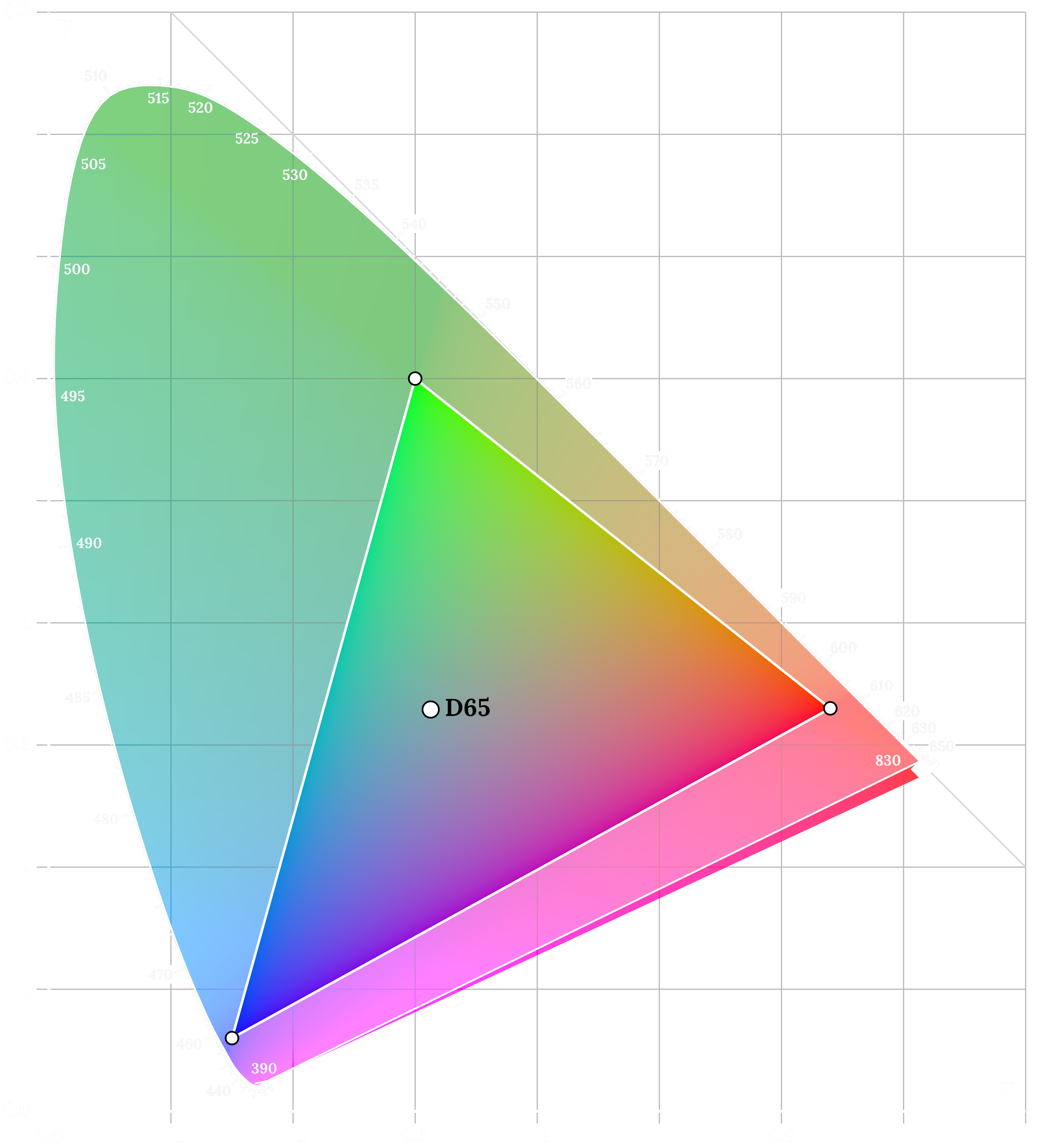
Figure 2
: The CIE xy diagram and the triangular "gamut" within it that can be displayed by the sRGB color standard. Note: the gamut is approximate; the chart is based on 2006 data, but sRGB's gamut coordinates are referred to 1931 data; see[19]. (Image by me.)Chromaticity
You can normalize the \(\vecinline{X,Y,Z}\) tristimulus triple (whether absolute XYZ or relative XYZ, the result is the same):
\[ \begin{bmatrix}x\\y\\z\end{bmatrix} = \begin{bmatrix}X\\Y\\Z\end{bmatrix} \bigg/ (X+Y+Z) \]The combination of \(x\), \(y\), and \(Y\) (the \(z\) is dropped) forms the
The \(\vecinline{x,y}\) coordinates are the space of color (color is therefore two-dimensional!), and the third coordinate \(Y\) represents brightness, as above.
The perimeter of the horseshoe-shaped region corresponds to spectra with only one wavelength—i.e. the rainbow, the most saturated colors you can see. The rainbow is the 1D boundary of the 2D region of color, and therefore (fun fact) the rainbow contains exactly 0% of all color by area!
Any point in the xy chart is called a '
Displays and Colors
At this point, we have converted our radiometric spectrum into the \(\vecinline{X,Y,Z}\) tristimulus triple representing, indirectly, the actual responses of cone cells within the human eye. Now, we need to transform it so that we can induce those responses, or at least some semblance of those responses, by setting pixels to certain colors.
This implements a 'portal' effect. You want your image of your rendered world to be seen by the viewer as if they were looking at it physically. This basically means that the real-world radiance emitted from the screen is (a metamer for) the radiance you are simulating in the virtual world.
While the idea is straightforward, the reality is that there are many different ways to do this because modern displays (though amazing) simply are unable to reproduce the richness of the real world. (Enter
Adding to the complexity: because everything is terrible, screens will often do their own thing instead of producing repeatable colors. For example, a typical phone screen will brighten and darken, and will oversaturate colors on-purpose to make them look more "vibrant". While this is arguably more visually appealing, it is usually uncontrollable, making correct reasoning about formal Colorimetry somewhere between challenging and impossible.
RGB Color-spaces and sRGB
Almost all color displays (including projectors as well as screens) are based on RGB color-spaces, of which there are many. Essentially every color display today supports a color standard called sRGB[21]. The best way I've found to think about sRGB is that it encompasses both a color-space and an encoding—that is, a description of the colorimetric properties of the system and a way of representing it in bytes[22].
While sRGB is an old standard and new screens can do much better, sRGB is also ubiquitous. By this point sRGB is so dominant that better color-spaces are finding it hard to gain programmatic traction, especially outside of cinema. Alternate RGB software APIs are currently clunky, platform-specific, and obscure—so sRGB conversion, while basic, is still the primary way we get pixels on the screen today. The attractiveness of sRGB is that you can blast three bytes per pixel onto nearly any screen in existence and get something reasonable out. There is currently no equivalent for more modern color-spaces, superior though they may be in theory.
In short, the sRGB standard is the sine qua non of display technology and RGB color-spaces (for better or for worse). And happily, all the other RGB color-spaces are defined through a very similar formalism. Therefore, we will study sRGB in detail as a running example.
RGB color-spaces are defined at minimum by three '
The primaries form a triangle in chromaticity space, which is the RGB color-space's '
The '
However, we do also at least need to know the related fact of how bright the white-point can be. For sRGB, the specified luminance is \(80~\unitsnit\)[25]. This is fairly dim and data can easily exceed this (e.g. a picture of the Sun would be \(1.6\times 10^9~\unitsnit\)). The sRGB standard says such values should be clipped[23], or we can add an additional factor of dimming, which we can think of as an exposure value. There's also tonemapping, as above. None of this is colorimetrically sound, but human observers get the point regardless.
In any case, note again that the brightness is not considered part of the definition of the white-point (nor of D65, which again has no units[24]). I suppose this encourages comparison of white-points between color-spaces with wildly different luminances.
sRGB Conversion: XYZ to ℓRGB
The three primaries, the white-point, and luminance are used to calculate a matrix[26] \(M\), whose inverse \(M^{-1}\) intuitively transforms \(\vecinline{X,Y,Z}\) into linear \(\vecinline{R,G,B}\) (which I call "ℓRGB" for clarity—a usage that seems to be gaining traction). It is 'linear' RGB to contrast with the final sRGB, which has a nonlinear gamma encoding (next section).
The actual transformation is widely seen online in a form that is simplified to the point of error (or at least contextual uselessness). The transformation matrix does indeed transform from ℓRGB to XYZ, but it is relativeXYZ. That is, RGB white has XYZ coordinate \(Y=1\). True, this seems like the most natural way to convert the spaces in isolation, but the detail of the scaling is almost always overlooked, nearly as often omitted from reference material, ends up adding computational overhead that could have been avoided by appropriate units, and has nontrivial implications about how scene luminance must be handled that are never explained. (I explain it all in detail at the link above.)
The practical point is that you must take your scene's spectral radiance, compute the absolute XYZ values from that, and then these XYZ values must all be normalized by a certain scaling factor, which I call \(\eta\). Wherefore, the actual transformation:
\[ \text{ℓRGB} = \begin{bmatrix}R\\G\\B\end{bmatrix} ~~=~~ \left( M^{-1} \right) \left( \eta \begin{bmatrix}X\\Y\\Z\end{bmatrix} \right) \]Where:
\[ M^{-1} ~~\approx~~ \begin{bmatrix} \phantom{-}3.2406 & - 1.5372 & - 0.4986\\ - 0.9689 & \phantom{-}1.8758 & \phantom{-}0.0415\\ \phantom{-}0.0557 & - 0.2040 & \phantom{-}1.0570 \end{bmatrix} \]That matrix is the 'official' version from the sRGB specification; a more-precise matrix can be computed using the definitions and linked algorithm above, if you prefer that. (This is indeed what I myself do, though I'm not sure I recommend it in general, as the results will be (very slightly) different from the standard. They will also be more colorimetrically accurate though, so . . . 🤷)
sRGB Conversion: ℓRGB to sRGB (Gamma Encoding)
The final step of sRGB conversion is to convert the ℓRGB triple of floating-point values into the sRGB triple of bytes. There's obviously a quantization, but there's also a nonlinear transformation called the
The gamma transform is pretty simple, though much nonsense has been written about it too. Basically, when we convert from a float to a byte, we lose a lot of precision. Each byte has only has 256 possible values, so we need to be careful about how we allocate that coding space. The human visual system is sensitive to proportional changes, so in particular it is very sensitive to changes in dim values. Therefore, it makes sense to allocate more of our limited codepoints to that region, by applying a nonlinear transform before quantizing. The gamma transform is this nonlinearity. (The screen is of course then engineered[28] to undo this transformation, so that the original real luminance is still displayed.)
In sum: we apply the inverse gamma transform to the linear floating-point data to make it nonlinear and more codepoints near zero, quantize to bytes, and send it to the screen. The display hardware then applies the forward gamma transform, converting the nonlinear data into linear (true) brightnesses. These linear brightnesses are interpreted by the human visual system in a way where the quantization inaccuracy is spread more evenly over the range of brightnesses.
The particular transformation the sRGB standard uses is a combination of a power law and a linear bias[29]. The specifics aren't very interesting; see the link for particulars. But, to save you (and me!) the trouble, here are implementations in Python and C++ that do the conversions:
1
2
3
4
5
6
7
8
9
10
11
12
13
14
15
16
17
18
19
20
21
22
23
24
25
26
27
28
29
30
31
class lRGB:
	def __init__( self, r:float,g:float,b:float ):
		self.r=r; self.g=g; self.b=b
class sRGB:
	def __init__( self, r:int  ,g:int  ,b:int   ):
		self.r=r; self.g=g; self.b=b

# gamma + quantization
def srgb_gamma_encode( val:float ):
	assert val >= 0.0
	if val >= 1.0      : return 255
	if val <= 0.0031308: val = 12.92 * val
	else               : val = 1.055*pow(val,1.0/2.4) - 0.055
	return int(round( 255.0 * val ))
# unpack and inverse gamma
def srgb_gamma_decode( val:int   ):
	tmp = float(val) / 255.0
	if tmp <= 0.04045: return tmp / 12.92
	else:              return pow( (tmp+0.055)/1.055, 2.4 )

# conversions between sRGB and lRGB
def lrgb_to_srgb( lrgb:lRGB ):
	r = srgb_gamma_encode(lrgb.r)
	g = srgb_gamma_encode(lrgb.g)
	b = srgb_gamma_encode(lrgb.b)
	return sRGB( r, g, b )
def srgb_to_lrgb( srgb:sRGB ):
	r = srgb_gamma_decode(srgb.r)
	g = srgb_gamma_decode(srgb.g)
	b = srgb_gamma_decode(srgb.b)
	return lRGB( r, g, b )
1
2
3
4
5
6
7
8
9
10
11
12
13
14
15
16
17
18
19
20
21
22
23
24
25
26
27
28
29
30
31
32
33
34
35
36
37
38
39
40
41
42
43
44
45
46
47
48
49
50
51
52
53
54
55
56
57
58
59
60
61
62
63
#include <cassert>
#include <cmath>
#include <cstdint>

struct lRGB final { float   r, g, b; };
struct sRGB final { uint8_t r, g, b; };

// gamma + quantization
[[nodiscard]] constexpr uint8_t srgb_gamma_encode( float   val ) noexcept
{
	assert( val >= 0.0f ); // Note catches NaN too.
	#if 0
		if ( val >= 1.0f ) return 255;
		val = val<0.0031308f ? val*12.92f : 1.055f*std::pow(val,1.0f/2.4f)-0.055f;
		return (uint8_t)std::round( 255.0f * val );
	#else
		if      ( val >= 1.0f       ) [[unlikely]] return 255;
		else if ( val <= 0.0031308f ) [[unlikely]] val *= 255.0f*12.92f;
		else [[likely]]
		{
			val = std::pow( val, 1.0f/2.4f );
			val = std::fma( 255.0f*1.055f,val, 255.0f*-0.055f );
		}
		return (uint8_t)std::round(val);
	#endif
}
// unpack and inverse gamma
[[nodiscard]] constexpr float   srgb_gamma_decode( uint8_t val ) noexcept
{
	#if 0
		float tmp = (float)val / 255.0f;
		tmp = tmp<0.04045f ? tmp/12.92f : std::pow((tmp+0.055f)/1.055f,2.4f);
		return tmp;
	#else
		float tmp = (float)val;
		if ( val <= 10 ) [[unlikely]] // `tmp <= 0.04045f*255.0f`
		{
			tmp *= (float)( 1.0 / (12.92*255.0) );
		}
		else [[likely]]
		{
			tmp = std::fma( (float)(1.0/(1.055*255.0)),tmp, (float)(0.055/1.055) );
			tmp = std::pow( tmp, 2.4f );
		}
		return tmp;
	#endif
}

// conversions between sRGB and lRGB
[[nodiscard]] constexpr sRGB lrgb_to_srgb( lRGB const& lrgb ) noexcept
{
	uint8_t r = srgb_gamma_encode(lrgb.r);
	uint8_t g = srgb_gamma_encode(lrgb.g);
	uint8_t b = srgb_gamma_encode(lrgb.b);
	return { .r=r, .g=g, .b=b };
}
[[nodiscard]] constexpr lRGB srgb_to_lrgb( sRGB const& srgb ) noexcept
{
	float r = srgb_gamma_decode(srgb.r);
	float g = srgb_gamma_decode(srgb.g);
	float b = srgb_gamma_decode(srgb.b);
	return { .r=r, .g=g, .b=b };
}
Note that the C++ version includes a simple implementation and an optimized implementation. Modern architectures have FMA instructions (compile with "-mfma"), so it makes sense to specify that we do the scale and bias with FMA—the compiler probably won't give you this automatically even with high optimizations[30]. We also, of course, replace the divisions by reciprocal multiplication, and combine some constants. Admittedly, these basic optimizations are somewhat futile; the slowest part by far is the power function—which is actually quite difficult to optimize without losing an unacceptable amount of precision. I'm working on a version that's much faster, but as yet it's more complicated and still only approximate.
Here's some test code to demo gamma encoding / decoding: