geometrian.comDoing the math, so you don't have to.
Light Transport, the Right Way
The familiar rendering equation is the basis of pathtracing, but it appears to lack a certain symmetry: the cosine term is only in one direction, and it is not clear how one would adapt it for bidirectional pathtracing.
The area form of the light transport equation is better, but the first point is privileged in the notation, and gives an output in radiance, which isn't the final radiometric quantity. To convert it, one needs to use the measurement equation, which mixes sample weights, importance, and reconstruction all together. These equations are less well known, and the measurement equation in particular is so rarely found that most graphics professionals don't even know it's supposed to exist.
In short, everything is all mixed up and confused. Putting it all together might be a lot to take in, but it would be all in one place and treated consistently!
The Fix
To fix this mess, you can take the area form of the light transport equation, substitute it into the measurement equation, converting the angular integration into an area integration. It turns out this magically fixes all the notational problems and makes everything intuitive.
Hence, I propose the following single equation that unifies everything[1]. Please don't be scared, even though it looks complex. It's actually extremely simple and more intuitive than any of the individual equations separately. I'll explain how, and give complete examples.
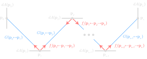
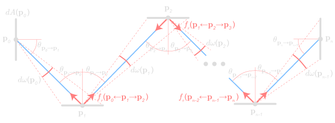
And here is the geometry for a given, arbitrary \(n\):
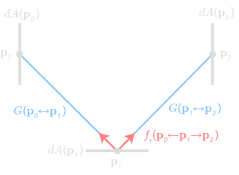
In case you're not familiar with it, \({\color{colorbrdf} f_r(\cdots)}\) is the bidirectional reflectance distribution function (BRDF). It is a property of the surface's material that describes how light reflects off of it. In more generality, we can consider all scattering (the BSDF), including light transmitted through the material.
\({\color{colorgeom} G(\cdots)}\) is a geometric coupling term, defined as:
The term \(V(\cdots)\) is the visibility function, which is \(0\) if \(\pt_k\) and \(\pt_{k+1}\) can't see each other and \(1\) if they can. Let's assume it's always \(1\) for the rest of this page, since if it's ever \(0\), then the whole \(\Phi_n\) is also \(0\).
The equation basically says that the radiant power (\(\Phi\)) arriving on the leftmost surface is the sum of all the radiant power arriving along paths of different lengths (\(\Phi_1\), \(\Phi_2\), ...).
Then, to compute the radiant power \(\Phi_n\) arriving along all paths of length exactly \(n\), we integrate over the \(n+1\) surfaces involved in that path. What do we integrate? The product of:
The BRDF \({\color{colorbrdf} f_r(\cdots)}\) of all interior nodes.
The geometric coupling terms \({\color{colorgeom} G(\cdots)}\) on all spans.
The radiometric quantity in question, which can be either:
The radiance \(L_e(\cdots)\) emitted from a light.
Importance \(W_e(\cdots)\) emitted from a sensor.
It takes the exact same place in the equation, because these are adjoint quantities (hey, symmetry!)
That's it. The power along a path is just the multiplied material and geometric terms, integrated over the surfaces involved.
Examples
Now, let's see how this can be used to derive some classic algorithms.
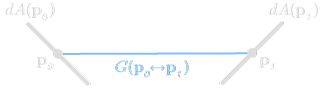
Simple Transport (\(\Phi_1\))
The above equation and geometry for \(\Phi_1\) is just:
Notice that there are no BRDF \({\color{colorbrdf} f_r(\cdots)}\) terms because there are no interior nodes.
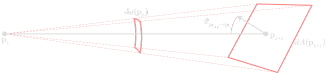
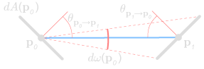
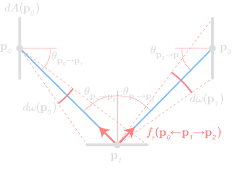
If we want, we can convert this to an integral over only the left-most surface by converting the sampling of the other surface \(\A{1}\) into a sampling over solid angle \(\Omega(\pt_0)\) from the first surface.
Recall the following identity from differential geometry:
Again, if we want the angular form, we can apply the same identity as in the previous example, twice; once each on \(\A{1}\) and \(A(\pt_2)\) to get \(\Omega(\pt_0)\) and \(\Omega(\pt_1)\), respectively. This gives:
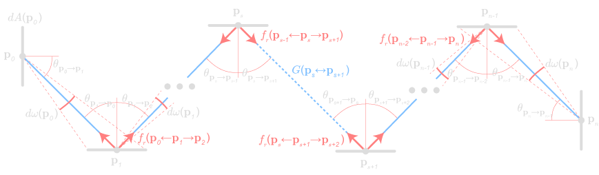
In bidirectional pathtracing, we generate one subpath from the eye (\(\pt_0,\pt_1,\cdots,\pt_e\)) and one subpath from the light (\(\qt_0,\qt_1,\cdots,\qt_l\)). These are then connected in the middle to form a single path (\(\pt_0,\pt_1,\cdots,\pt_e,\qt_l,\qt_{l-1},\cdots,\qt_0\)).
We relabel this so that it's a contiguous range (\(\pt_0,\pt_1,\cdots,\pt_s,\pt_{s+1},\cdots,\pt_n\)), where the split is between \(\pt_s\) and \(\pt_{s+1}\). When we do this, the exact original area equation from the top of the page applies (we're sampling over area either way, regardless of which subpath a new node was first connected to)!
For the angular form, however, we have to be a little more careful. Point \(\pt_s\) is sampled, as in standard pathtracing, from point \(\pt_{s-1}\). However, point \(\pt_{s+1}\) is sampled in the other direction, from \(\pt_{s+2}\). Therefore, the angles between \(\pt_s\) and \(\pt_{s+1}\) do not matter in the sampling (although they do matter for the geometry term that remains to connect them).