Introduction to the Rendering Equation
David Immel et al. and James "Jim" Kajiya simultaneously introduced the rendering equation into graphics in 1986. Most online formulations suffer from poor notation, a lack of intuition, and a lack of examples. This page is my attempt to explain it properly, showing how it can be adapted to the usual Monte Carlo methods we use in graphics.
For simplicity, \(\lambda\) (wavelength), \(t\) (time), transparency, volumetrics, and subsurface effects are not included in this formulation. My notation will be somewhat more verbose because explicitness aids clarity. For integrating color, see here, and for a more advanced treatment of path space, see here.
The Rendering Equation
First, you have to know what the rendering equation looks like and what it does. Simply put, the rendering equation defines how much light leaves from any point in a 3D scene in a given direction. Most surfaces simply reflect light, but others (also) emit it. Putting this into more mathematical language: the outgoing light from a given point in a particular direction is the sum of the amount of light it emits in that direction and the amount of light it reflects in that direction from any incoming light:
\begin{align*} \newcommand{wi}{\vec{\omega}_i} \newcommand{wo}{\vec{\omega}_o} \definecolor{colorL}{RGB}{255,255,128} \definecolor{colorG}{RGB}{128,192,255} \definecolor{colorBRDF}{RGB}{255,128,128} \definecolor{colordefl}{RGB}{221,221,221} \newcommand{canceldefl}[2]{ \color{colordefl} \cancel{\color{#2}#1} } {\color{colorL} L_o(\vec{x},\wo) } ~~&=~~ {\color{colorL} L_e(\vec{x},\wo) } + {\color{colorL} L_r(\vec{x},\wo) }\\ ~~&=~~ {\color{colorL} L_e(\vec{x},\wo) } + \int_{ \Omega(\vec{x},\vec{N}) } {\color{colorL} L_o(\vec{y}_i,\,-\wi) } ~ {\color{colorG} |\vec{N}\dotprod\wi| } ~ {\color{colorBRDF} \vec{f}_r(\vec{x},\wi,\wo) } ~ d\wi \end{align*}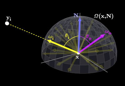
Figure 0
: Geometry of the rendering equation. For every possible \(\wi\), we add up how much of the incoming light (from point \(\vec{y}_i\) in that direction) reflects toward the (fixed) direction of interest \(\wo\).We have a point \(\vec{x}\) on a surface, with normal \(\vec{N}\). On the left-hand-side, we want to find the light \({\color{colorL} L_o(\vec{x},\wo) }\) coming out of \(\vec{x}\) along a given, fixed, outgoing direction \(\wo\). Formally, the units are radiance[1] (intuitively, the 'brightness'). You may also see it written e.g. \(L_o(\vec{x}\rightarrow\wo)\), which is slightly nonstandard, but perhaps more descriptive.
Obviously, any light the surface emits in that direction, \({\color{colorL} L_e(\vec{x},\wo) }\), is counted (only light sources emit; for other surfaces, this is just zero). However, the more complicated thing to compute is how much light reflects, \({\color{colorL} L_r(\vec{x},\wo) }\), and that's what the integral does. Light can arrive from any incoming direction \(\wi\), and then scatter along the outgoing direction of interest \(\wo\). So, the idea of the integral is to sum up the reflection contribution from all possible directions \(\wi\) in the hemisphere[2][3] \(\Omega(\vec{x},\vec{N})\) above the surface.
Note: \(\wo\) and \(\wi\) are both from the hemisphere, and in particular \(\wi\) points oppositely from the direction the light arrives at the surface. This convention makes sense with more theory, and especially when considering more advanced bidirectional techniques, but can be confusing if you weren't expecting it. Just remember that the incoming light propagates along \(-\wi\).
The inside of the integral has three terms. First, we have another radiance term, \({\color{colorL} L_o(\vec{y}_i,\,-\wi) }\), which is the incoming light from direction \(\wi\). It takes the form of the outgoing light from another point \(\vec{y}_i\). Basically, we look out from \(\vec{x}\) along \(\wi\) and find the surface point \(\vec{y}_i\) that that direction hits; the outgoing light from \(\vec{y}_i\) along \(-\wi\) is then the same as the incoming light to \(\vec{x}\) from \(\wi\). This outgoing light can be computed by using the whole equation again, recursively! If there is no surface in direction \(\wi\), the term can be zero or some value from an environment map, forming the base case of the recursion.
The second term, \({\color{colorG} |\vec{N}\dotprod\wi| }\), is usually called the 'geometry term'. The best way to understand this is as a dimensionless correction factor, needed to convert the first term into a form usable by the third term. We'll discuss this more below. You will also often see this equivalently written as \(|\cos\theta_i|\), where \(\theta_i\) is the angle between \(\vec{N}\) and \(\wi\). It is also very common to (erroneously) drop the absolute value[4].
The third term, \({\color{colorBRDF} \vec{f}_r(\vec{x},\wi,\wo) }\), is the bidirectional reflectance distribution function (BRDF)[5], which describes how much light reflects from the incoming direction \(\wi\) along the outgoing direction \(\wo\). This determines how the light's reflection is distributed as it hits a surface—is it sharp and mirror-like? Or flatter and more diffuse, like paper? You will see it written with different arguments, or with arrows, e.g. as \(\vec{f}_r(\wi\leftarrow\vec{x}\rightarrow\wo)\).
Units and Differentials
The rendering equation can also be written in the form of differentials, or in SI units (integral part only, for clarity):
\begin{alignat*}{6} &{\color{colorL} L_r(\vec{x},\wo) } ~~&&=~~ \int_{ \Omega(\vec{x},\vec{N}) } && {\color{colorL} L_o(\vec{y}_i,\,-\wi) } ~ && {\color{colorG} |\vec{N}\dotprod\wi| } ~ && {\color{colorBRDF} \vec{f}_r(\vec{x},\wi,\wo) } ~ && d\wi \\ &{\color{colorL} \frac{d^2\Phi_{r}}{d\wo~dA~|\cos\theta_o|} } ~~&&=~~ \int_{ \Omega(\vec{x},\vec{N}) } && {\color{colorL} \frac{ \canceldefl{d^2\Phi_i}{colorL} }{ \canceldefl{d\wi}{colorL} ~ \color{colorL}dA ~ \canceldefl{|\cos\theta_i|}{colorL} } } ~ && \canceldefl{ |\cos\theta_i| }{colorG} ~ && {\color{colorBRDF} \frac{d^3\Phi_r}{ \canceldefl{d^2\Phi_i}{colorBRDF} ~ \color{colorBRDF}d\wo ~ |\cos\theta_o| } } ~ && \cancel{d\wi} \\ &{\color{colorL}\left[ \frac{\text{W}}{\text{sr}\cdot\text{m}^2} \right]} ~~&&=~~ \int_{ \Omega(\vec{x},\vec{N}) } && {\color{colorL}\left[ \frac{\text{W}}{\text{sr}\cdot\text{m}^2} \right]} ~ && \canceldefl{[ 1 ]}{colorG} ~ && \canceldefl{\left[ \text{sr}^{-1} \right]}{colorBRDF} ~ && \cancel{[\text{sr}]} \end{alignat*}Units and Differentials: the BRDF
The only somewhat difficult part here is the BRDF, \({\color{colorBRDF} \vec{f}_r(\vec{x},\wi,\wo) }\). The BRDF is formally the differential ratio of reflected (outgoing) radiance to incident (incoming) irradiance and, from that definition, we can figure the differentials[6]:
\begin{align*} \vec{f}_r(\vec{x},\wi,\wo) &= \frac{ d L_r(\vec{x},\wo) }{ d E_i(\wi) }\\ &= \frac{ d(~d^2\Phi_r~/~(d\wo~dA~|\cos\theta_o|)~) }{ d(~d\Phi_i~/~dA~) } = \frac{ d^3\Phi_r/(d\wo~dA~|\cos\theta_o|) }{ d^2\Phi_i/dA }\\ &= \frac{ d^3\Phi_r }{ d^2\Phi_i ~ d\wo ~ |\cos\theta_o| } \end{align*}Meanwhile, the BRDF's units are just radiance divided by irradiance, which works out to be \(\left[\text{sr}^{-1}\right]\) just from cancellation:
\[ \vec{f}_r(\vec{x},\wi,\wo) = \left[\frac{ \text{W}/(\text{sr}\cdot\text{m}^2) }{ \text{W}/\text{m}^2 }\right] = \left[\text{sr}^{-1}\right] \]The BRDF must satisfy several key properties. First, its value must always be nonnegative (since light cannot be negative). Second, it must exhibit Helmholtz reciprocity, which in this context basically means that for any given pair of directions \(\wi\) and \(\wo\), you can swap them and the function value is the same. Third, the cosine-weighted integral over its domain must be exactly \(1\), so that energy is neither created nor destroyed:
\[ \int_{ \Omega(\vec{x},\vec{N}) } {\color{colorG} |\vec{N}\dotprod\wi| } ~ {\color{colorBRDF} \vec{f}_r(\vec{x},\wi,\wo) } ~ d\wi ~~=~~ 1,\hspace{1cm}\text{(for all $\wo$)} \]It should be noted that this last criterion is often extremely difficult to ensure, so it is common to relax it into a \(\leq\). This corresponds to energy loss, but at least not energy gain[7]. Spurious absorption is a necessary evil at best, but at least it's not spurious amplification.
Units and Differentials: the Geometry Term
Let's dig a little more into the geometry term, \({\color{colorG} |\vec{N}\dotprod\wi| = |\cos\theta_i|}\). As above, the geometry term is a dimensionless correction term. We can now see how it arises: it is needed to cancel the corresponding quantity in the denominator of the first term.
A higher level way to see the same result is to look at the BRDF again. The denominator \(d E_i(\wi)\) of the BRDF can actually be written in terms of radiance[8]:
\[ d E_i(\wi) = L_o(\vec{y}_i,\,-\wi) ~ |\cos\theta_i| ~ d\wi \]Thus we can cancel differently, without expanding the first term:
\[ {\color{colorL} L_r(\vec{x},\wo) } ~~=~~ \int_{ \Omega(\vec{x},\vec{N}) } \canceldefl{ L_o(\vec{y}_i,\,-\wi) ~ \color{colorG} |\cos\theta_i| }{colorL} ~ {\color{colorBRDF} \frac{ d L_r(\vec{x},\wo) }{ \color{colordefl} \canceldefl{ L_o(\vec{y}_i,\,-\wi) ~ |\cos\theta_i| }{colorBRDF} ~ \canceldefl{ d\wi }{colorBRDF} } } ~ \cancel{d\wi} \]
Figure 1
: Light spreading out due to angle results in more or less irradiance, explaining why the poles are colder and (with tilt) the seasons. (Image modified from Wikipedia.)
Intuitively, the geometry term accounts for the attenuation of incoming light due to falling on an angled surface: the radiance coming in from shallower angles gets spread over a larger \(dA\), and so needs to be attenuated. This kind of attenuation is exactly what that dot product term does.
This is actually the same effect that gives Earth its climate (see Figure 1). A beam of light from the sun is spread out over more area nearer to the poles, meaning that the ground receives less light per square meter, and therefore less warmth. Thus, the poles are generally cold, while the equator is generally hot.
The Earth's tilt adds an additional layer, causing the seasons. When a hemisphere tilts away from the sun, the angle is steeper, and so the light is more spread out and you get winter, while when the hemisphere tilts toward the sun, the angle is shallower, and so the light is more concentrated and you get summer.
It's actually possible to go even further: just as the geometry term \({\color{colorG} |\cos\theta_i| }\) attenuates the incoming light, we can consider the outgoing light to be scaled by \(1/|\cos\theta_o|\). In previous versions of this tutorial, I called this the 'explicit' formulation (to contrast with the standard formulation, which I called 'implicit'), and worked through examples.
Although the mathematics is consistent either way, the price paid is that the definition of the BRDF must be changed. The new BRDFs are incompatible with standard analysis, and also tend to be more complicated. They also lack the Helmholtz reciprocity property stated above, so they aren't even truly 'bidirectional' anymore. For these reasons, I recommend against doing light transport in this way.
Summary and Next Steps
The rendering equation describes how much light leaves a surface in a given direction, and is the sum of the emitted light and the reflected light. The reflected light is gathered from all incoming directions by an integral of three terms: the incoming radiance, computed recursively, a dimensionless geometry term to handle light spreading, and a BRDF, which describes how the reflected light is distributed.
I also offer related tutorials on:
- Using Monte Carlo techniques with the rendering equation, the most direct follow-on to this tutorial.
- Advanced light transport, including bidirectional techniques, through the area formulation of the light transport equation.
- Radiometry and colorimetry, with in-depth explanation of terms like 'radiance'.