Monte Carlo Rendering Equation
The rendering equation, introduced in my tutorial here, describes how light bounces around the scene:
\begin{align} \newcommand{wz}{\vec{\omega}_z} \newcommand{wik}{\vec{\omega}_{ i,k }} \newcommand{wi}[1][]{\vec{\omega}_{ {#1}i }} \newcommand{wo}[1][]{\vec{\omega}_{ {#1}o }} \definecolor{colorL}{RGB}{255,255,128} \definecolor{colorG}{RGB}{128,192,255} \definecolor{colorBRDF}{RGB}{255,128,128} {\color{colorL} L_o(\vec{x},\wo) } ~~&=~~ {\color{colorL} L_e(\vec{x},\wo) } + {\color{colorL} L_r(\vec{x},\wo) } \nonumber \\ ~~&=~~ {\color{colorL} L_e(\vec{x},\wo) } + \int_{ \Omega(\vec{x},\vec{N}) } {\color{colorL} L_o(\vec{y}_i,\,-\wi) }~ {\color{colorG} |\vec{N}\dotprod\wi| }~ {\color{colorBRDF} \vec{f}_r(\vec{x},\wi,\wo) }~ d\wi \label{eq:reneqn} \end{align}Unfortunately, it is a recursive integral equation, and is usually impossible[1] to solve in closed-form. Fortunately, there is another way to solve integrals: Monte Carlo integration. As explained in my tutorial here, an integral can be calculated with:
\begin{equation} \text{Let }x_k \sim \pdf(x)\text{. Then } E\!\left[ \frac{g(x_k)}{\pdf(x_k)} \right] = \int_{domain} g(x)~ d x\text{.} \label{eq:mcint} \end{equation}where \(E[\cdots]\) denotes expected value (the average of a random variable) and \(\pdf(\cdots)\) is a probability density function (a function that says the probability density of choosing its argument, naturally therefore integrating to \(1\) over its domain). Basically, we can sample a random \(x_k\) according to \(\pdf(x)\) and, on average, \(g(x_k)/\pdf(x_k)\) will be the correct value of the integral. Actually, we can literally do that average, by taking many samples \(x_k\) and averaging them.
This tutorial describes some of the complexities of applying Monte Carlo integration to the rendering equation, and gives examples for some BRDFs.
Solving the Rendering Equation with Monte Carlo Integration
The obvious first step is to combine \(\eqref{eq:reneqn}\) and \(\eqref{eq:mcint}\):
\begin{equation} {\color{colorL} L_o(\vec{x},\wo) } ~~=~~ {\color{colorL} L_e(\vec{x},\wo) } + E\!\left[ {\color{colorL} L_o(\vec{y}_i,\,-\wik) }~ {\color{colorG} |\vec{N}\dotprod\wik| }~ {\color{colorBRDF} \vec{f}_r(\vec{x},\wik,\wo) }~ \frac{1}{\pdf(\wik)} \right] \label{eq:mcreneqn} \end{equation}Just to be clear what this means: the random variable is the direction \(\wi\). We sample a value \(\wik\) out of the hemisphere, weighted according to some distribution \(\pdf(\wi)\), and evaluate the integrand. The expected value of the right-hand-side is then the answer to the integral. (Note: we compute the incoming radiance \(L_o(\vec{y}_i,\,-\wik)\) recursively, as discussed below, but it doesn't really change any of the following analysis. Just pretend it's a known constant.)
Lambertian BRDF, with Uniform Sampling
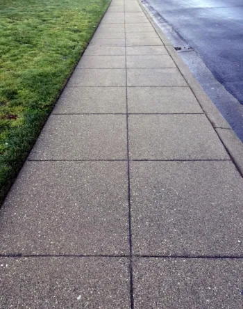
Figure 0
: Squares on a sidewalk appear more numerous with distance, but are also more inclined. The two effects cancel, and the sidewalk looks roughly a constant color. (Image modified from fostercity.org.)The most basic case is the Lambertian BRDF:
\[ {\color{colorBRDF} \vec{f}_r(\vec{x},\wi,\wo) } ~~\defeq~~ {\color{colorBRDF} \frac{\rho_d}{\pi} } = {\color{colorBRDF} k_d } ,\hspace{1cm}0 \leq \rho_d \leq 1 \]The Lambertian BRDF is the simplest BRDF: literally just a constant. It seems most sensible to define it as above, with \(\rho_d\) the albedo and \(k_d\) the overall constantkonstant, though sometimes you'll see it backward[3].
Notice that it is a valid BRDF because it fulfills the criteria: it is nonnegative, it is the same when you swap the arguments, and its cosine-weighted integral is \(\leq 1\) (actually, it's exactly \(\rho_d\)):
\begin{align*} \int_{ \Omega(\vec{x},\vec{N}) } {\color{colorG} |\vec{N}\dotprod\wi| }~ {\color{colorBRDF} \vec{f}_r(\vec{x},\wi,\wo) }~ d\wi ~~&=~~ {\color{colorBRDF} \frac{\rho_d}{\pi} } \int_{ \Omega(\vec{x},\vec{N}) } {\color{colorG} |\vec{N}\dotprod\wi| }~ d\wi \\ ~~&=~~ {\color{colorBRDF} \frac{\rho_d}{\pi} }~ \pi \\ ~~&=~~ \rho_d ~~\leq~~ 1,\hspace{1cm}\text{(for all $\wo$)} \end{align*}Meanwhile, the simplest possible sampling is a uniform distribution, selecting directions uniformly at random from the unit hemisphere. The unit hemisphere has surface area \(2\pi\) (it's half that of a sphere), so the probability density is \(1/(2\pi)\):
\[ \pdf(\wi) ~~\defeq~~ \frac{1}{2\pi} \]With these definitions, we can substitute into the Monte Carlo form of the rendering equation, \(\eqref{eq:mcreneqn}\) and get:
\begin{align*} {\color{colorL} L_o(\vec{x},\wo) } ~~&=~~ {\color{colorL} L_e(\vec{x},\wo) } + E\!\left[ {\color{colorL} L_o(\vec{y}_i,\,-\wik) }~ {\color{colorG} |\vec{N}\dotprod\wik| }~ {\color{colorBRDF} \frac{\rho_d}{\pi} }~ \frac{1}{ 1/(2\pi) } \right]\\ ~~&=~~ {\color{colorL} L_e(\vec{x},\wo) } + 2~ \rho_d~ E\!\left[~ {\color{colorL} L_o(\vec{y}_i,\,-\wik) }~ {\color{colorG} |\vec{N}\dotprod\wik| } ~\right] \end{align*}Not bad! We simply multiply the incoming light by twice the albedo and the geometry term, and recurse to compute the next \(L_o\) with a \(\wik\) chosen uniformly at random from the hemisphere!
Lambertian BRDF, with Importance Sampling
We can do better, however. It turns out that the Monte Carlo method converges faster when you choose your random samples from a distribution that 'looks like' the integrand; this is called 'importance sampling'. That is, although we can choose any shape we like for \(\pdf(\wi)\), it behooves us to make it proportional to the integrand, \({\color{colorL} L_o(\vec{y}_i,\,-\wi) }~ {\color{colorG} |\vec{N}\dotprod\wi| }~ {\color{colorBRDF} \rho_d/\pi }\).
We unfortunately can't do anything about the \(L_o\), because we don't know it, but nothing stops us from choosing \(\pdf(\wi)\) according to the rest (though we drop the \(\rho_d\) because \(\pdf(\wi)\) must always integrate to \(1\)):
\[ \pdf(\wi) ~~\defeq~~ \frac{|\vec{N}\dotprod\wi|}{\pi} \]That is, we now choose our random \(\wik\) from a cosine-weighted hemisphere, instead of a uniformly weighted hemisphere.
With this change, we can now substitute into \(\eqref{eq:mcreneqn}\) and get:
\begin{align*} {\color{colorL} L_o(\vec{x},\wo) } ~~&=~~ {\color{colorL} L_e(\vec{x},\wo) } + E\!\left[ {\color{colorL} L_o(\vec{y}_i,\,-\wik) }~ {\color{colorG} |\vec{N}\dotprod\wik| }~ {\color{colorBRDF} \frac{\rho_d}{\pi} }~ \frac{1}{ |\vec{N}\dotprod\wik|/\pi } \right]\\ ~~&=~~ {\color{colorL} L_e(\vec{x},\wo) } + \rho_d~ E\!\left[~ {\color{colorL} L_o(\vec{y}_i,\,-\wik) } ~\right] \end{align*}This is even simpler, and it converges faster, too! It really is this simple. For example, check out the SmallPT example pathtracer; you'll see this formula used on line 60, along with the required cosine-weighted hemisphere sampling just above.
Specular BRDFs (Case Study: Modified Phong)
The Modified Phong[4][5] BRDF is probably the simplest specular BRDF that isn't just a mirror. It takes the form:
\[ {\color{colorBRDF} \vec{f}_r(\vec{x},\wi,\wo) } ~~\defeq~~ {\color{colorBRDF} \frac{\rho_s}{I_M} \max(~ 0, R(\wi,\vec{N})\!\dotprod\!\wo ~)^n } \]where \(\rho_s\) is the albedo, \(I_M\) is the energy normalization term, \(R(\wi,\vec{N})\) is a function that reflects \(-\wi\) off the plane defined by \(\vec{N}\), and \(n\) is a nonnegative real parameter called the 'specular exponent'.
The basic idea is that you take the incoming light direction \(\wi\), calculate how it would reflect if the surface were a mirror, find how close that is to the actual outgoing direction \(\wo\) by using the dot product, and then raise it to some power to change how significant that similarity is considered to be.
We can of course use this BRDF to do Monte Carlo integration. For the \(I_M\) in the sidebar and uniform hemisphere samples, the same technique as before gives us:
\begin{align*} {\color{colorL} L_o(\vec{x},\wo) } ~~&=~~ {\color{colorL} L_e(\vec{x},\wo) } + E\!\left[ {\color{colorL} L_o(\vec{y}_i,\,-\wik) }~ {\color{colorG} |\vec{N}\dotprod\wik| }~ {\color{colorBRDF} \frac{n+2}{2\pi}~ \rho_s~ \max(~ 0, R(\wik,\vec{N})\!\dotprod\!\wo ~)^n }~ \frac{1}{ 1/(2\pi) } \right]\\ ~~&=~~ {\color{colorL} L_e(\vec{x},\wo) } + (n+2)~ \rho_s~ E\!\left[~ {\color{colorL} L_o(\vec{y}_i,\,-\wik) }~ {\color{colorG} |\vec{N}\dotprod\wik| }~ \max(~ 0, R(\wik,\vec{N})\!\dotprod\!\wo ~)^n ~\right] \end{align*}and for cosine-weighted hemisphere samples, we get:
\begin{align*} {\color{colorL} L_o(\vec{x},\wo) } ~~&=~~ {\color{colorL} L_e(\vec{x},\wo) } + E\!\left[ {\color{colorL} L_o(\vec{y}_i,\,-\wik) }~ {\color{colorG} |\vec{N}\dotprod\wik| }~ {\color{colorBRDF} \frac{n+2}{2\pi}~ \rho_s~ \max(~ 0, R(\wik,\vec{N})\!\dotprod\!\wo ~)^n }~ \frac{1}{ |\vec{N}\dotprod\wik|/\pi } \right]\\ ~~&=~~ {\color{colorL} L_e(\vec{x},\wo) } + \left( \frac{n+2}{2} \right)~ \rho_s~ E\!\left[~ {\color{colorL} L_o(\vec{y}_i,\,-\wik) }~ \max(~ 0, R(\wik,\vec{N})\!\dotprod\!\wo ~)^n ~\right]\\ \end{align*}Although the latter is better, unfortunately, neither of these importance-samples the BRDF very well. Many of the samples \(\wik\) will reflect to a vector \(R(\wik,\vec{N})\) that is not close enough to \(\wo\) to have a very large dot product, or power of dot product, or even positive value at all. These samples constitute work we have to do, yet don't contribute to the integral's value.
To improve this, we need to importance sample in the direction the BRDF is strongest. This is a difficult problem, but we can get partially there. Consider a random variable \(\wz\), a direction from a power of a cosine lobe centered around \(\vec{z}=\vecinline{0,0,1}\), and then rotate this so it is distributed around \(R(\wo,\vec{N})\) instead. That is, we sample[6][7] vector \(\vec{\omega}_{z,k}\) around \(\vec{z}\) according to the distribution:
\[ \pdf(\wz) ~~\defeq~~ \frac{n+1}{2\pi}~ |\wz\dotprod\vec{z}| \]and then rotate it by \(\cos^{-1}(R(\wo,\vec{N}) \dotprod \vec{z})\) around axis \((\vec{z}\times R(\wo,\vec{N}))/||\vec{z}\times R(\wo,\vec{N})||\) to center the distribution around \(R(\wo,\vec{N})\), giving us our distribution for \(\wi\):
\[ \pdf(\wi) ~~=~~ \frac{n+1}{2\pi}~ |\wi\dotprod\wo| \]Sampling from this gives our \(\wik\), and the Monte Carlo estimate:
\begin{align*} {\color{colorL} L_o(\vec{x},\wo) } ~~&=~~ {\color{colorL} L_e(\vec{x},\wo) } + E\!\left[ {\color{colorL} L_o(\vec{y}_i,\,-\wik) }~ {\color{colorG} |\vec{N}\dotprod\wik| }~ {\color{colorBRDF} \frac{n+2}{2\pi}~ \rho_s~ \max(~ 0, R(\wik,\vec{N})\!\dotprod\!\wo ~)^n }~ \frac{1}{ |\wik\dotprod\wo|~ (n+1)/(2\pi) } \right]\\ ~~&=~~ {\color{colorL} L_e(\vec{x},\wo) } + \left( \frac{n+2}{n+1} \right) \rho_s~ E\!\left[~ {\color{colorL} L_o(\vec{y}_i,\,-\wik) }~ \left|\frac{ \vec{N}\dotprod\wik }{ \wik\dotprod\wo }\right|~ \max(~ 0, R(\wik,\vec{N})\!\dotprod\!\wo ~)^n ~\right]\\ \end{align*}There are two issues that make this imperfect, however. The first is that we aren't importance sampling the geometry term anymore, so the convergence is still not ideal. However, this will still be better, at least when the specular exponent \(n\) is large. To importance-sample both terms at once, we need to use multiple importance sampling, the subject of perhaps a future tutorial.
The second issue is that when we rotate \(\wz\), it can actually end up underneath the ecliptic plane, and therefore not be a valid reflection direction (so the BRDF value is zero). You can't really improve on that; flipping it above the ecliptic plane or generating a new sample will bias or double-count the distribution.
Monte Carlo Pathtracing
Finally, a quick detour into the gist of how this fits into an overall renderer.
A Monte Carlo solution to the rendering equation almost invariably means the renderer is a 'forward pathtracer', which is a specific kind of raytracing renderer. (There are other kinds of pathtracer, but forward is the commonest and, with a few concessions, arguably the best.)
A forward pathtracer starts by tracing a ray from the eye until it hits an object. The rendering equation applies: to compute the light exiting back toward the eye, we need to add the emission and the reflection. The reflection is computed with the integral. Instead of trying to solve the integral in closed-form, we simply sample a single direction \(\wik\) and try to find the light coming back along that. We trace the ray until we reach another surface, where the rendering equation applies again. And so on.
At each step, we compute the integral by looking for the light coming from a single direction, recursively. We continue until we decide to stop (the ray leaves the scene, it hits a surface of albedo zero, we reach some maximum depth, etc.). In effect, we are substituting the rendering equation into itself recursively[8]:
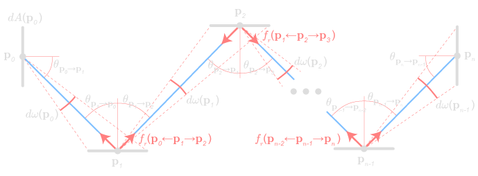 \begin{align*} {\color{colorL} L_{0,o} } ~~&=~~ {\color{colorL} L_{0,e} } + \int_{\Omega_0} {\color{colorL} L_{1,o} }~ {\color{colorG} |\cos\theta_0| }~ {\color{colorBRDF} \vec{f}_{0,r} }~ d\wi[0,] \\ ~~&=~~ {\color{colorL} L_{0,e} } + \int_{\Omega_0} \left( {\color{colorL} L_{1,e} } + \int_{\Omega_1} {\color{colorL} L_{1,o} }~ {\color{colorG} |\cos\theta_1| }~ {\color{colorBRDF} \vec{f}_{1,r} }~ d\wi[1,] \right)~ {\color{colorG} |\cos\theta_0| }~ {\color{colorBRDF} \vec{f}_{0,r} }~ d\wi[0,] \\ ~~&=~~ {\color{colorL} L_{0,e} } + \int_{\Omega_0} \left( {\color{colorL} L_{1,e} } + \int_{\Omega_1} \left( {\color{colorL} L_{2,e} } + \int_{\Omega_2} {\color{colorL} L_{2,o} }~ {\color{colorG} |\cos\theta_2| }~ {\color{colorBRDF} \vec{f}_{2,r} }~ d\wi[2,] \right)~ {\color{colorG} |\cos\theta_1| }~ {\color{colorBRDF} \vec{f}_{1,r} }~ d\wi[1,] \right)~ {\color{colorG} |\cos\theta_0| }~ {\color{colorBRDF} \vec{f}_{0,r} }~ d\wi[0,] \\ ~~&\vdots \end{align*}
 When we apply Monte Carlo integration, the integrand is really the inside of all of these integrals. We trace only the single[9][10] path through the scene, and that's the estimate. However, at a functional level, this is all sortof obvious, and the code is essentially unchanged.
I have a teaching pathtracing renderer, which is a basic but real example, and may be of interest.