CS 6620.001 "Ray Tracing for Graphics" Fall 2014
Welcome to my ray tracing site for the course CS 6620.001, being taught at the University of Utah in Fall 2014 by Cem Yuksel.
Welcome fellow students! I have lots of experience tracing rays, and with graphics in general, and so I'll be pleased to help by giving constructive tips throughout (and I'll also try very hard to get the correct image, or say why particular images are correct as opposed to others). If you shoot me an email with a link to your project, I'm pretty good at guessing what the issues in raytracers are from looking at wrong images.
Hardware specifications, see bottom of page.
Timing information will look like "(#t #s ##:##:##)" and corresponds to the number of threads used, the number of samples (per pixel, per light, possibly explained in context), and the timing information rounded to the nearest second.
Project 10 - "Soft Shadows and Glossy Surfaces"
My renderer has supported correct glossy reflections, complete with correct importance sampling, for a very very long time. In fact, the difficult part heretofore has been not using them (much)! The reflections are based on a Phong lobe and can be varied so as to conserve energy with this nasty formula I once derived for a paper (since significantly improved and published):
\[ \begin{align*} \gamma &= \arccos\left(\vec{V}\cdot\vec{N}\right)\\ T_i &= \begin{cases} \pi & \text{if } i=0\\ 2 & \text{if } i=1\\ \frac{i-1}{i}T_{i-2} & \text{otherwise} \end{cases}\\ F_o&=\frac{1}{n+1}\left[ \pi +\cos(\gamma)\sum\limits_{m=0}^{n-1}\sin^{2m }(\gamma)T_{2m }\right]\\ F_e&=\frac{1}{n+1}\left[2(\pi-\gamma)+\cos(\gamma)\sum\limits_{m=0}^{n-1}\sin^{2m+1}(\gamma)T_{2m+1}\right] \end{align*} \]In the above, \(\gamma\) is the angle \(\vec{V}\) makes with \(\vec{N}\) and \(n\) is the (integer-valued) specular exponent. \(F_o\) and \(F_e\) are the normalization terms for \(n\) odd or even, respectively.
This allows the following images to exist; without them, energy would be lost as the specular lobe approaches the ecliptic. People generally consider this loss to be good because it models shadowing in a microfacet BRDF. Unfortunately, it ignores multiple scattering. The correct answer is somewhere in-between.
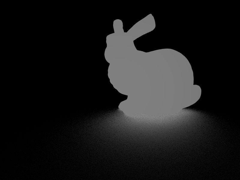
These images have been resized by half for space; view the originals for full detail! Specular exponent \(n:=3\); (16t 16,^2s 00:03:26):
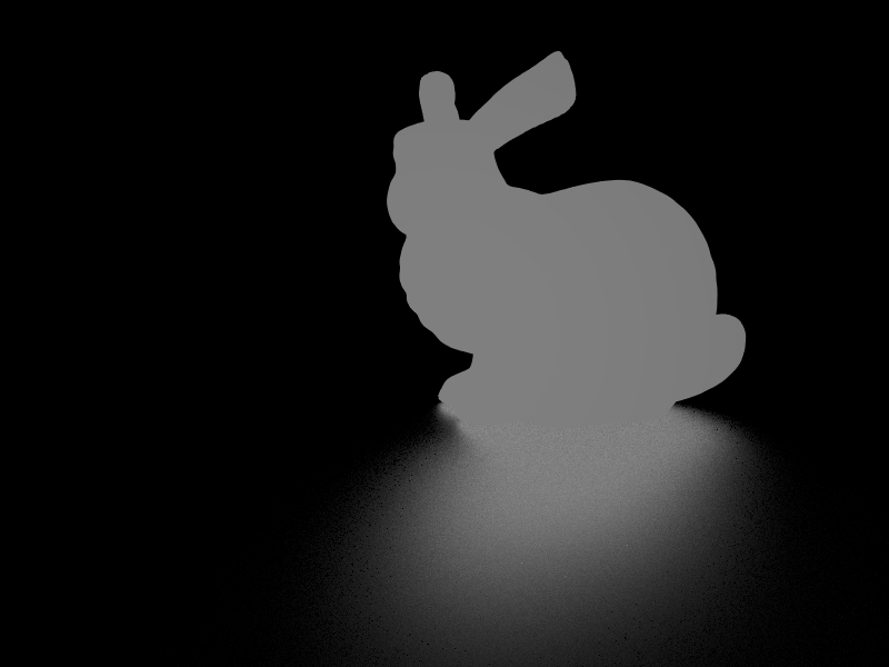
Specular exponent \(n:=30\); (16t 16,^2s 00:03:49):
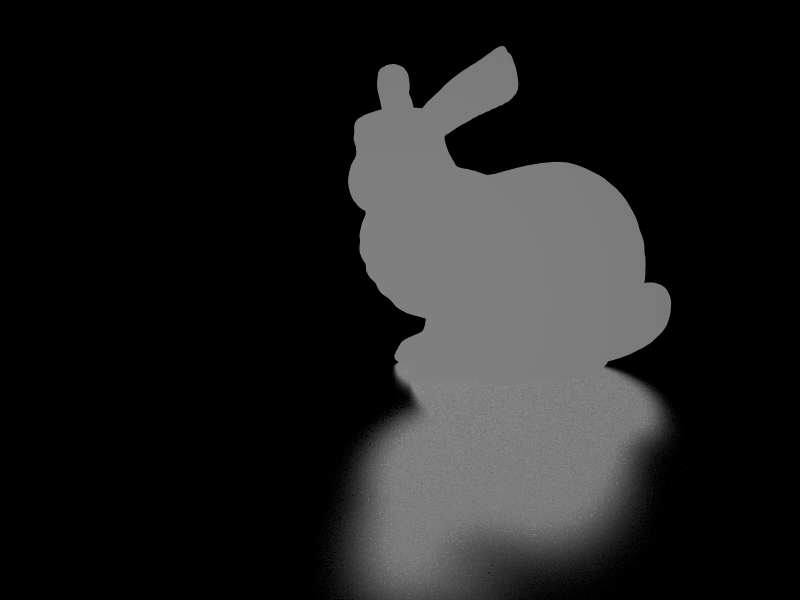
Specular exponent \(n:=300\); (16t 16,^2s 00:02:45):
Specular exponent \(n:=3000\); (16t 16,^2s 00:01:20):

Specular exponent \(n:=30000\); (16t 16,^2s 00:00:55):

Specular exponent \(n:=300000\); (16t 16,^2s 00:00:51):

Specular exponent \(n:=3000000\); (16t 16,^2s 00:00:51):

The last one, in particular, took a long time to set up. This is because the computation of the normalization factors is not memoized, and therefore \(O(n^2)\). Notice that, because we're normalizing, these images converge nicely toward a delta function ignoring the geometry term (and each reflection has the same energy—a handy feature). The edges are very faintly darker too; this comes from using a correct camera model.
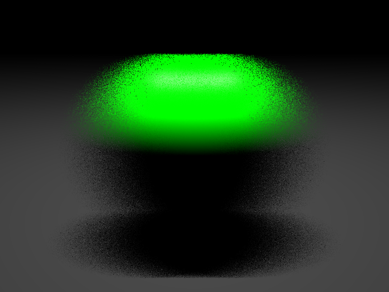
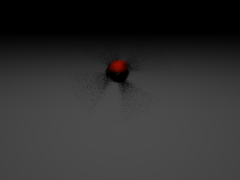
The other thing to notice is that triangle lights are supported. So are spheres. Other implicit surfaces (e.g. the fractals from project 3) can't be lights because there isn't a nice way to find their total radiant flux (which I require of all lights). Planes are nonmanifold and infinite, and so would emit infinite flux (which is a problem for light-emitting algorithms). I do support axis-aligned boxes, but I'm having some issues integrating them fully. I just need to give them a bit of attention, so I'm omitting the (incorrect) renders that show these objects being used as lights.
These renders needed to use naïve path tracing (i.e. no explicit light sampling), since every single triangle is an individual light source! You could sample toward a given triangle (light), but a lot of the time it would be occluded by another light and so would be in the shadow of the first light. Explicit light sampling can't reuse the shadow ray to do lighting coming from the shadowing surface (since that would be biased), so a lot of rays would be wasted. Instead, the ray just bounces randomly until it hits a surface, adding from the surface's emission function as necessary. This works wonderfully since the new ray direction is importance-sampled.
The other main thing I did was implement motion blur like I said I was going to. My implementation operates by interpolating transformation matrices, which is horrible but seems to be de rigueur. My implementation supports a stack of matrices, interpolated as frequently as you like, but the loader only supports two (the endpoints of the interval). Only a square-wave shutter is currently implemented.
Here's a simple test. The timing is what I remember (16t 4,^2s 00:00:47):
I loaded an airplane model (I finally found one that's kindof okay from here). I had to manually adjust the ".obj" file's ".mtl" file export, since it got all the textures wrong. Also, glass has two sides, so I had to fix some normals and extrude the canopy inward.
I figured out a nice camera position in Blender, but it took me several hours to figure out how to map it correctly to our scenefiles. The algorithm is to set the camera in "XYZ Euler" and then write transforms in your scenefile that look something like this:
<rotate x="1" degrees="90"/>

<!-- Negative of "Location" -->
<translate x="-0.73644" y="1.39943" z="-0.55620"/>
<!-- Negative of "Rotation"'s z-component -->
<rotate z="1" degrees="-37.463"/>
<!-- Negative of "Rotation"'s y-component -->
<rotate y="1" degrees="32.076"/>
<!-- Negative of "Rotation"'s x-component -->
<rotate x="1" degrees="-63.645"/>

<!-- [Object Follows] -->
Part of the problem was that Blender, like many other modeling softwares use \(\vec{z}\) for up, which at the time this was written I found to be deeply problematic.
Several tests were rendered, but the first of the airplane with a significant of samples looked like this (16t 4,^2s 01:19:11):
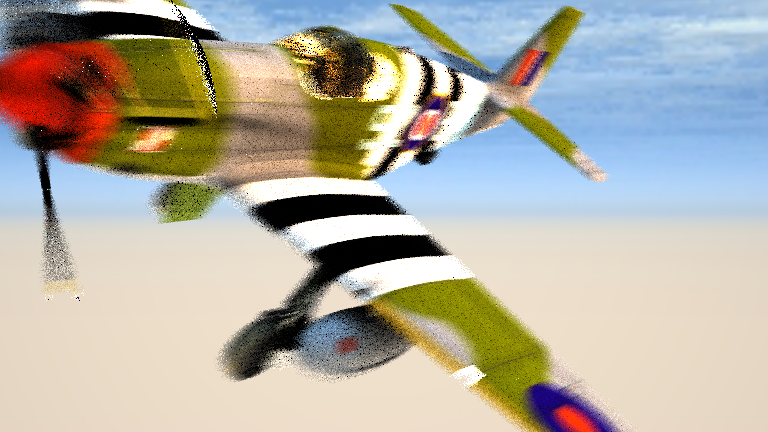
By far the longest part of rendering this image was the airplane (the background probably would have taken only a few seconds by itself). Since triangles take up more room when blurred and are more expensive to transform, throwing the maximum \(64\) samples per pixel took a long time. Of the airplane, the most expensive part was the glass, which required an obscene amount of time, and (because the simplest inside path is \(ESSDSSL\)) still got undersampled.
To get the motion blur on the propeller, it was exported as a separate ".obj", and also given a rotational blur of \(30^{\circ}\). Unfortunately, this winds up being too slow relative to the rest of the airplane. The canopy is a third ".obj", but the ".mtl" material is overridden with my own physically-based glass material.
There's full environment mapping here. There's a fill light off to the side, but much of the illumination comes from the environment, (which is importance-sampled, as all lights in my renderer can be, of course). You can see this on some lighter parts of the aircraft, such as the wing.
The most objectionable artifact is the propeller rim, which was caused by an int overflowing from an extremely strong specular highlight. A simple fix.
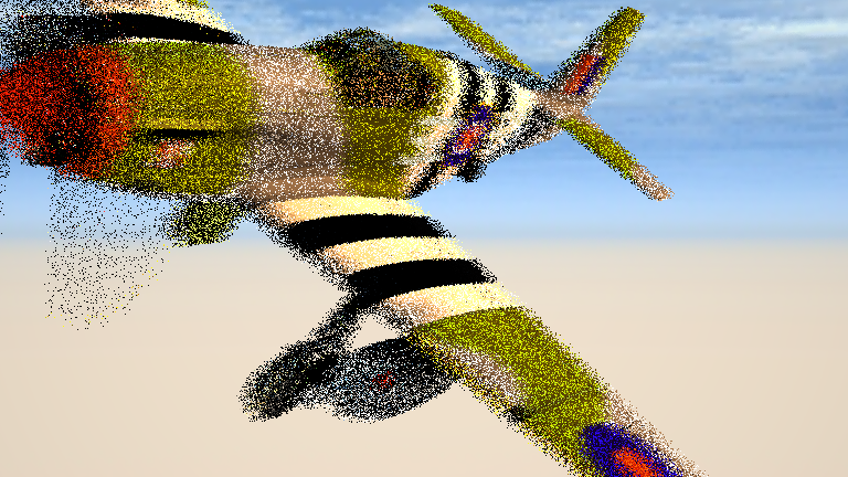
The rest was more problematic. I even had dreams about it. I eventually figured out that the transform to object space doesn't work for linearly blended rays (it actually magically becomes nonlinear), so instead you need to do the intersection in world space. I'll think about it more later, but doing it this way at least fixes the nonlinear effects (like the doubled roundel insigne on the side of the airplane). I also patched the loader to be able to handle any number of interpolation points. After fixing some glitches (which took way too long) I got this simple test (16t 2,^2s 00:00:38):
This uses three points of interpolation (so two steps). With that, it's time for another render. Here's the airplane again, but with only one sample per pixel. I tripled the speed of the propeller (up to \(90^{\circ}\)) using the newly improved rotations (using eight points; seven steps). (16t 1,^2s 00:00:32):
For the next render I adjusted the sample count and resolution and halved the linear velocity. This render is resized by half. View the original in full HD! (16t 16,^0s 00:42:25):

More samples! This render is also resized by half. View the original in full HD! (16t 32,^0s 01:24:07):

Bleh . . . I think these used my Whitted renderer instead of path tracing with explicit light sampling . . .
Here's the actual assignment, using ELS path tracing (16t 16,^0s 00:02:17):

More samples (16t 64,^0s 00:08:50):
Proceed to the Previous Project or Next Project.
Hardware
Except as mentioned, renders are done on my laptop, which has:
- Intel i7-990X (12M Cache, [3.4{6|7},3.73 GHz], 6 cores, 12 threads)
- 12 GB RAM (DDR3 1333MHz Triple Channel)
- NVIDIA GeForce GTX 580M
- 750GB HDD (7200RPM, Serial-ATA II 300, 16MB Cache)
- Windows 7 x86-64 Professional (although all code compiles/runs on Linux)