CS 6620.001 "Ray Tracing for Graphics" Fall 2014

Welcome to my ray tracing site for the course CS 6620.001, being taught at the University of Utah in Fall 2014 by Cem Yuksel.

Welcome fellow students! I have lots of experience tracing rays, and with graphics in general, and so I'll be pleased to help by giving constructive tips throughout (and I'll also try very hard to get the correct image, or say why particular images are correct as opposed to others). If you shoot me an email with a link to your project, I'm pretty good at guessing what the issues in raytracers are from looking at wrong images.

Hardware specifications, see bottom of page.

Timing information will look like "(#t #s ##:##:##)" and corresponds to the number of threads used, the number of samples (per pixel, per light, possibly explained in context), and the timing information rounded to the nearest second.

Project 11 - "Monte Carlo GI"

Like many of the previous projects, I've had indirect illumination implemented for a long time. I suppose I don't actually have a special configuration set up for just the single bounce expected, but that's because it's sortof trivial and boring. My implementation does full path tracing already. So, I spent this project working on improving various other features of my raytracer.

First, I implemented spectral rendering. Spectral rendering (where each ray additionally has a wavelength associated with it) is fairly straightforward to think about, but more complex to actually implement in a renderer that's based on non-spectral rendering. Fortunately, I had done a lot of the implementation already, and I just had to finish it up.

The first problem I encountered after implementing it was that, when cranking up the samples, my framebuffer implementation couldn't handle it past a certain point. This is because the memory required can become ridiculous. For example, one of my test scenes (from SmallPT) for dispersion (an effect only possible with spectral rendering, caused by the index of refraction varying with wavelength) is $1024 \times 768 \times 1000$ (XGA $1000$ samples per pixel). With each sample being stored in "double"s and with associated metadata for each sample, even with only three wavelength buckets, it works out to $29$ GiB of data! This clearly doesn't fit in my laptop's RAM.

So, the first thing I did was rewrite the framebuffer implementation, again. This turned out to be surprisingly easy (although it took longer than it should have; I kept procrastinating because I thought it wasn't going to be easy). The implementation is now cruftier than I'd like, but it works. I also fixed the black background issue (wasn't setting alpha) and implemented reconstruction filtering (currently supporting box, Mitchell–Netravali, and Lanczos windowed sinc).

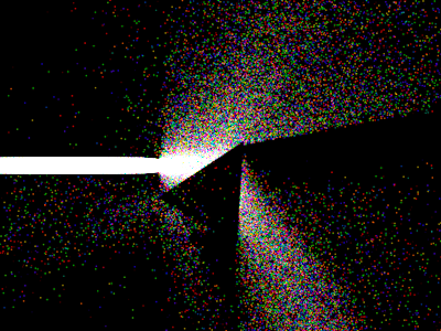
Here's a rendering in progress. The checker pattern is untouched pixels, the magenta pixels are pixels being sampled, the yellow pixels are pixels that have enough samples, but haven't been reconstructed, the green-overlaid pixels are reconstructed pixels awaiting deallocation of their sample data (so that everything fits in RAM) and the other pixels (that are the rendered color) are entirely-completed pixels:

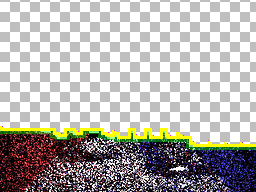
The implementation here is kindof protracted. Since the deallocation of a pixel's samples can't be done until all of the other pixels that depend on that pixel have been reconstructed, and since the reconstruction of a pixel's samples can't be done until all of the other pixels that depend on that pixel have been sampled, a naïve implementation would be ridiculously complex. The way I solve this is by delegating the reconstruction and deallocation to two different threads that constantly cycle over all the pixels in a scene. In practice, this eats a surprisingly small amount of CPU time, and the render threads never get far ahead. It's messy and suboptimal, but it works quite well in practice. Note: I shall not count these threads in the thread count for timing statistics.

Here are some different filters on the scene for project 7 and project 8. All were rendered using path tracing with explicit light sampling.

Box (16t 4,^0s 00:00:42):

Rendering using box reconstruction filtering.

Mitchell–Netravali ($B=0.350$, $C=0.325$) (16t 4,^0s 00:00:38):

Rendering using Mitchell–Netravali reconstruction filtering.

Lanczos windowed sinc (cutoff $2$) (16t 4,^0s 00:00:37):

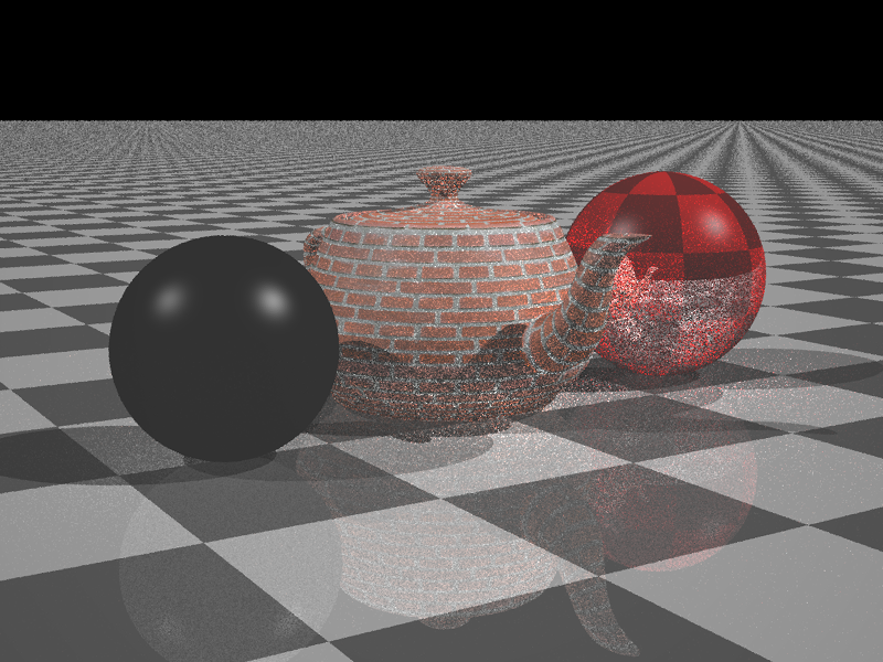
Rendering using Lanczos reconstruction filtering (cutoff 2).

Lanczos windowed sinc (cutoff $3$) (16t 4,^0s 00:00:42):

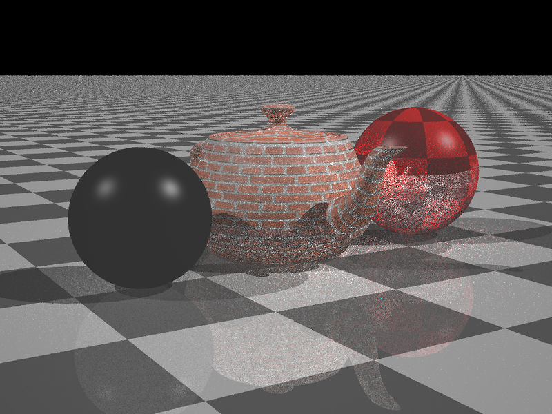
Rendering using Lanczos reconstruction filtering (cutoff 3).

Note that there is some faint ringing especially on the windowed sinc. From these results, I am selecting Mitchell–Netravali as the default filter.

A side-effect of all this is that the deallocation is now taking a long time again. It will have to do for now.

Without further ado, here's some with/without (cropped to rendered area) dispersion images. Note the extra bluish hue around the edge of the caustic:

Without (16t 1000,^0s 00:06:08)	With (16t 1000,^0s 00:06:00)

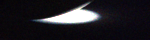I don't think the slight decrease in rendering time is insignificant; the tracer is heavily optimized, and with spectral rendering there are slightly fewer computations that need to be done for each ray.

Those are wrong. They aren't being scaled by the PDF of choosing the wavelength, and I'm pretty sure they aren't colorimetric.

Colorimetry is the study of how radiometry is perceived. I have a tutorial on the basics. Long story short, after finding the radiant flux at a pixel, you convert it to CIE XYZ (defining how it appears) and then from there into sRGB (defining how to display it to get that appearance). I had already implemented a lot of this, but it took some work to get right. In particular, you need to be careful when combining colors: it's the radiometric spectra that must be averaged, not the final sRGB values.

Also, since we're now no longer visualizing radiometric spectra, things that were "white" or "red" or whatever now are much more complicated. Here's a white plane rendered under a flat emission spectrum (i.e. constant spectral radiant flux from $390nm$ to $700nm$ discretized over six spectral buckets) (no timing data available, but I think it was around a minute or so for each):

Direct (16t 100,^0s 00:??:??)	Spectral (16t 100,^0s 00:??:??)

They look the same. That's the point.

Also, notice that the plane appears somewhat reddish. I suspect this is because most emission spectra aren't constant—and blackbody radiation, which approximates many light sources (especially the sun and incandescent bulbs) reasonably well, emits more in the blue side. If anyone has some actual, reproducible data on how various surfaces look like under various simple emission spectra, I'd love to see it!

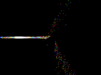
I tried to set up a prism to get good dispersion effects. The following is the first one I threw a decent number of samples at (16t 1000,^0s 00:27:17), 16 spectral buckets:

Unsatisfactory spectral rendering of prism.

The light source is a vertical quad surrounded by two walls to channel it into a beam. There are several problems here. The first is that the walls are made out of the same material as the floor—a highly reflective Lambert material. In fact, except for light lost out the top and for bias, all the light comes out the front end of the channel, the minority in a collimated manner. This also slows the render, since no early termination can be done for these paths. The second problem is that even the collimated light is too spread out. You can see this in the shadow of the prism.

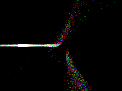
I let this render run to completion just for show, but it's really not worth much. Here's a rerender with narrower, nonreflective walls, and fewer samples (16t 100,^0s 00:01:38):

More samples (16t 1000,^0s 00:27:21):

Clearly, this is really a job for something like photon mapping. Trying to sample this with forward path tracing is a terrible idea.

It's time to improve importance sampling. Currently, Blinn–Phong BRDFs aren't importance sampled (I didn't know how) and importance sampling generally wasn't taking into account the geometry term.

Blinn–Phong can be importance sampled by importance sampling a Phong lobe centered around the normal, and then using that as the half vector $\vec{\omega}_\vec{H}$. When paired with the first vector $\vec{\omega}_i$, you can find the second vector $\vec{\omega}_o$. You need to be careful, though. The PDF you get from sampling $\vec{\omega}_\vec{H}$ is not the same as that you'd get from sampling $\vec{\omega}_o$! You need to transform the PDF. I found this which states that the transformation function needs to be monotonic (which doesn't make sense in spherical coordinates, really!). I presume they meant "injective", in which case we're fine because the transformation mapping

\[ \vec{g}(\vec{\omega}_i,\vec{\omega}_\vec{H}):=\vec{R}(\vec{\omega}_i,\vec{\omega}_\vec{H}) = -\vec{\omega}_i+2\left(\vec{\omega}_i\cdot\vec{\omega}_\vec{H}\right)\vec{\omega}_\vec{H}= \vec{\omega}_o \]

. . . happens to be bijective in $\vec{\omega}_i \times \vec{\omega}_o$ space! I worked on figuring out what the transformation should be for a while (way too long), but I couldn't get anything useful. However, it turns out that Physically Based Rendering has the final answer, which they derive through a trigonometric argument (pg.697–698) as:

\[ \pdf_{\vec{\Omega}_i}\left(\vec{\omega}_i\right) = \frac{ \pdf_{\vec{H}}\left(\vec{\omega}_{\vec{H}}\right) }{ 4\left(\vec{\omega}_i\cdot\vec{\omega}_{\vec{H}}\right) } = \frac{ \pdf_{\vec{H}}\left(\vec{\omega}_{\vec{H}}\right) }{ 4\left(\vec{\omega}_o\cdot\vec{\omega}_{\vec{H}}\right) } \]

As far as the geometry term, the only BRDF I know where you can actually take it into account directly is the Lambert BRDF. Let me know if you know of others!

Here's a table of renders from the various BRDFs showing the effect of importance sampling. The scene is a "perfectly reflective" plane with the given BRDF covered by an emitting dome. Note that the BRDFs are not in general "perfectly reflective". The Blinn–Phong model loses energy, and so does the Phong model without the correction I invented (see project 10). The Lambertian BRDF is simple enough to lose no energy.

BRDF	No Importance Sampling	Importance Sampling
Lambertian	(16t 10,^0s 00:00:04):	(16t 10,^0s 00:00:04):
Phong (exponent $10$)	(16t 10,^0s 00:00:03):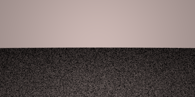	(16t 10,^0s 00:00:04):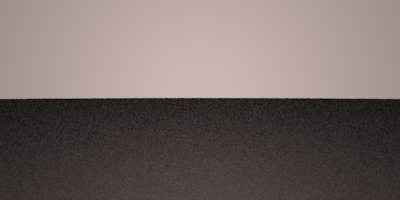
Phong (Energy Corrected) (exponent $10$)	(16t 10,^0s 00:00:03):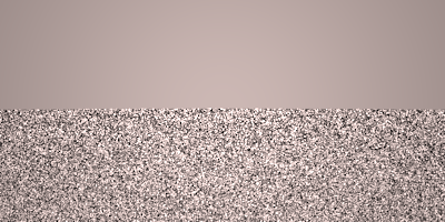	(16t 10,^0s 00:00:04):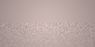
Blinn–Phong (exponent $10$)	(16t 10,^0s 00:00:04):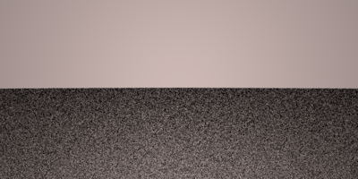	(16t 10,^0s 00:00:03):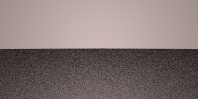

Here's the first image of the assignment (16t 100,^0s 00:17:53):

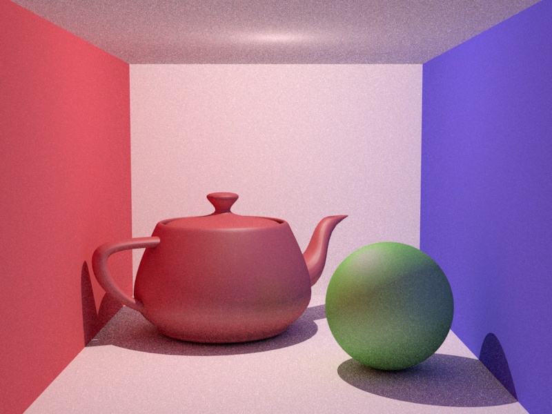
Rendering of required scene: a teapot and sphere in a Cornell box, including indirect light.

Amazingly, this looks very similar to the expected image.

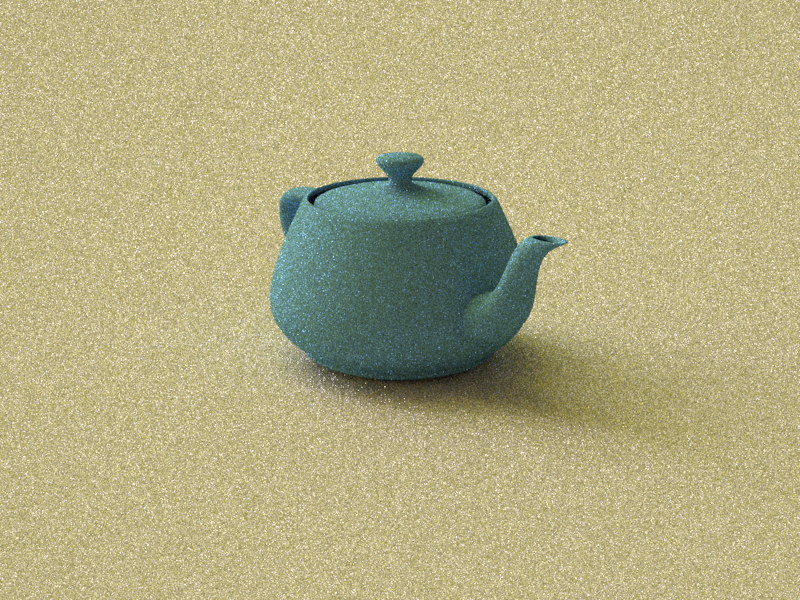
Here's the second image of the assignment (16t 100,^0s 00:05:29):

Rendering of required scene: a teapot on a plane, including indirect light.

You can get arguably nicer results using Lambertian with less albedo. I also changed the color to be pretty. This has exactly the same number of samples; for a huge area light like this, Lambertian gives less noise. (16t 100,^0s 00:05:35):

Here's using the "outdoor" environment map (which I thought was from Debevec, but apparently isn't; the only place I could find it was here—which might just be some site mirroring someone's work for a profit, since I didn't have to pay for the original). I also changed the algorithm from pathtracing to pathtracing with explicit light sampling (which importance samples the environment map) (16t 100,^0s 00:05:29):

This looks really realistic, especially from a distance—and it should! A real-world environment light is illuminating a Lambertian surface (reasonably realistic). The light is bouncing around potentially a large number of times, and then reflecting into a physically based camera. After being modulated by the camera's response curve, the signal is converted to CIE XYZ, which defines how it should appear to humans, and then modulates out an sRGB image, thus setting the pixels in the correct way to induce that appearance.

The only ways this could be improved are by using more samples with infinite (or RR) depth, using DOF (there was none here), or by using measured BRDFs. None of these are very important for this scene.

I spent a lot of Monday rebuilding a broken computer, but in the evening I had my computer render these tests:

No Spectral	Spectral ($64$ channels)
(16t 100,^0s 00:00:28)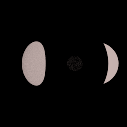 $RGB rendering of refractive sphere.$	(16t 100,^0s 00:01:06)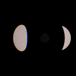 $Spectral rendering of refractive sphere.$
(16t 1000,^0s 00:06:03)	(16t 1000,^0s 00:07:04)

Interestingly, the majority of the expense was reconstruction. The first is a transparent sphere in front of a spherical light source, which it partially occludes. The second is a crop from SmallPT.

The refraction for both of these renders used "Dense Flint" (N-SF66) (data available from refractiveindex.info). I picked this because it has a very low Abbe number and very high refractive index (criteria for maximum dispersion). For the no-dispersion case, a constant approximation is used.

Here's a longer rerender I left going overnight (16t 5000,^0s 10:32:50):

Rendering of adjusted scene, with more samples.

Proceed to the Previous Project or Next Project.

Hardware

Except as mentioned, renders are done on my laptop, which has:

Intel i7-990X (12M Cache, [3.4{6|7},3.73 GHz], 6 cores, 12 threads)
12 GB RAM (DDR3 1333MHz Triple Channel)
NVIDIA GeForce GTX 580M
750GB HDD (7200RPM, Serial-ATA II 300, 16MB Cache)
Windows 7 x86-64 Professional (although all code compiles/runs on Linux)