CS 6620.001 "Ray Tracing for Graphics" Fall 2014

Project 6.5 - Misc. Changes

I know I said I would implement certain features first. I didn't.

First: photon mapping. I coded it up pretty quickly, but getting even half-passable results was difficult. I had a bunch of problems with the kNN (k nearest neighbors) photon sampling, mainly because std::priority_queue<...> is stupid and useless, and the std:: functions for heap operations work oddly.

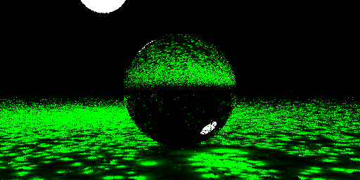
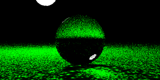
My very first photon mapped images (lots of problems, \(10^5\) photons and \(10^6\) photons) (16t 1s 00:00:20), (16t 1s 00:00:29):

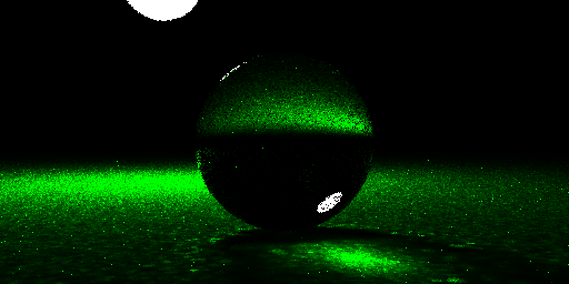
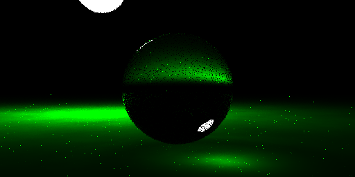
After I fixed a problem with the priority queue, it seemed to be working decently. There's obviously still some problems though. Resized images with timing information:

\(10^7\) samples with 10 photon gather, (16t 1s 00:08:20)	\(10^6\) samples with 500 photon gather, (16t 1s 00:03:15)	\(10^6\) samples with 50 photon gather, (16t 1s 00:00:50)

Part of the way I do graphics—or really anything—is to stumble around until I discover things. Then I push on these until I understand what they do and why. I'm a fast and good enough coder that this is almost as fast as just looking it up—but a whole lot more fun and lasting in memory. Of course, I also look stuff up occasionally—if only to check my progress.

Having pushed on photon mapping a while, I have learned the following:

• Photon maps should not be used for direct illumination. This is the main problem with the above images. Note: Jensen actually advocates separating into three photon maps: one for caustics, one for global illumination (meaning indirect diffuse bounces), and a volume photon map, as applicable. It appears he advocates exactly not using photon maps for direct illumination in §8.2.1 of Realistic Image Synthesis. So I was right.
• Since the non-specular surfaces you hit don't go in the photon map, if the secondary rays die a lot, you don't add any photons. So, you can use a huge number of primary photons since most of them will die. Importance sampling the caustic-generating, specular objects sounds like a great idea (Jensen advocates this too).
• Making your photon maps smaller makes the final gather go a lot faster. My KD-tree is optimized, but is not optimal for memory accesses, which is the biggest cost of accessing it. The photons are also allocated individually, and pointers are stored in the KD tree to make the entire structure smaller.
• The radius of the gather and the number of photons used matters a lot too—both to performance and to quality.
• More photons in an estimate makes your result blurry.

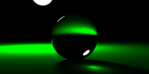
The main thing is the first point above. When fixing that (and a few other glitches that made their way in during refactoring) one gets (16t 10s 00:05:10) with \(10^6\) photons and \(100\) in the gather. Note: the photon map was cached for this render, so it didn't need to be generated.

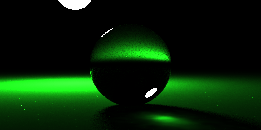
Well that's nice! I think the surface needs a little bit of red and blue reflection, and also let's use \(10^7\) primary photons and \(1000\) in the gather. I made an important optimization that limits the initial search region. This has the effect of preventing many photons from being entered into the priority queue only to be evicted later. The photon map was cached for this one too (and I realize I didn't make the plane reflect enough of the other colors). (16t 10s 00:04:50):

Alright, well that's nice. Time for some more interesting caustics! Let's revisit Lucy. In retrospect, one of the reasons the refraction project's Lucy looks weird was because her base was sticking out the bottom of the scene. Because of refractive priorities, rays could escape. I'm not sure of that, but just in case, I moved her up \(0.3\) units. Since last time, I also improved the way triangles are handled: there is no transformation cost anymore. I could have sworn I rendered an image (16t 10s 00:14:54) with a low resolution version of the model and cached photonmap, but I can't find it. My conclusion:

Blech. Lucy! You need stronger caustics, girl!

A smaller and more powerful light and less absorption in its spectrum should help. Also, I realized that the radiosity is actually being calculated twice: once by the path trace, and once by the diffusely reflected photons in the photonmap. I tweaked the photon map so that it doesn't continue any trace that hits a diffuse surface—so this is only a "caustics" photon map. This also allows one to use more photons, since the only photons that have any cost for rendering are the ones that hit Lucy (and those are the ones we want!). I tried all this, and I still couldn't get really visible caustics. Short of shooting a light through her face right up against a wall, I don't think this model is going to generate anything.

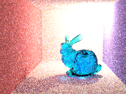
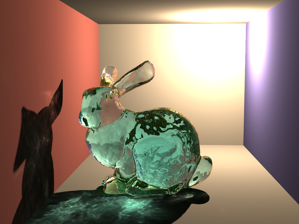
Boom. Bunny. \(100{,}000\) photons, \(10^5\) gather (16t 10s 00:01:30), including photon map generation this time:

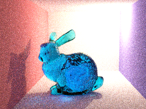
Same except \(10^6\) photons and tweaked scene (16t 10s 00:02:37):

One of the nice things about photon mapping is that if you cache the photons, you can reuse them. Here's the exact same data rendered at a higher resolution (16t 10s 00:09:50):

Here's a large render with \(10^8\) photons, \(100\) samples and \(10\) photon gather in a maximum radius of \(0.5\) (16t 100s 07:19:27):

The photon map that these images generate is kinda pretty. As I recall, this is from the larger render, and was about \(8\%\) generated:

My .obj file loader, which was one of the oldest parts of my graphics library, having gone through several major revisions/rewrites basically unscathed, hadn't aged well. In particular, for large files it would take a long time to load. This was mainly due to two related factors. First, the file was loaded into a std::list<...> of lines, incurring an allocation cost and the list overhead for each. Second, when the stack was popped, this list had to be deallocated, which could take on the order of minutes! Clearly, unacceptable.

So, Friday 26^th and Saturday 27^th I rewrote the parsing code, mostly from scratch. When it loads the file, it copies the data into a flat buffer with embedded metadata that implements a linked list. This required a lot of pointer arithmetic, reinterpret_casting, and even revealed a compiler bug. When reading, there's no real indirection that happens; you're just skipping around a flat buffer. Once this datastructure was built, it actually makes the process of doing the actual parsing easier.

To incorporate the new structure, I had to rewrite my parsers for ".stl" and ".obj" files. The ".obj" one in particular was painful, but I implemented some sophisticated features. For example, it only stores unique vertex data and unique vertex records. The old version tried to do this, poorly. This time, there's some fancy pre-cached hashing going on that allows duplicate marking to proceed efficiently.

After profiling out a few mostly minor optimizations, the average load time for \(1\%\) decimated Lucy (\(140{,}311\) vertices and \(841{,}668\) triangles) is \(0.4162\) seconds and \(1.248\) seconds, without and with duplicate removal, respectively. For my production code, duplicate removal is enabled. This is a massive speedup from previously.

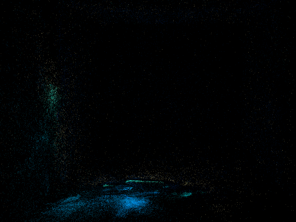
I reworked a bunch of the photonmapping code. The main part had been written at stupid-'o-clock in the morning, so the architecture needed a reboot. I added some snazzy (mostly) cross-platform font coloring and reworked the integrators' rendering phases into distinct queues. I also changed the minimum sample to \(8\) (Jensen's default) and tweaked the algorithm so that it would only render one diffuse bounce (i.e. no radiosity). The result (in a little under \(40\) minutes with eye and light specular depth \(64\) (sorry, no precision timing available)):

Now that's more like it! The photonmap was just gorgeous at various stages during its generation. Once it was completed, it was a bit washed out. Here's what it looked like after the photon map had been generated and the trace was underway. Notice that the photonmap was loaded from its cached file (I restarted it to make some changes):

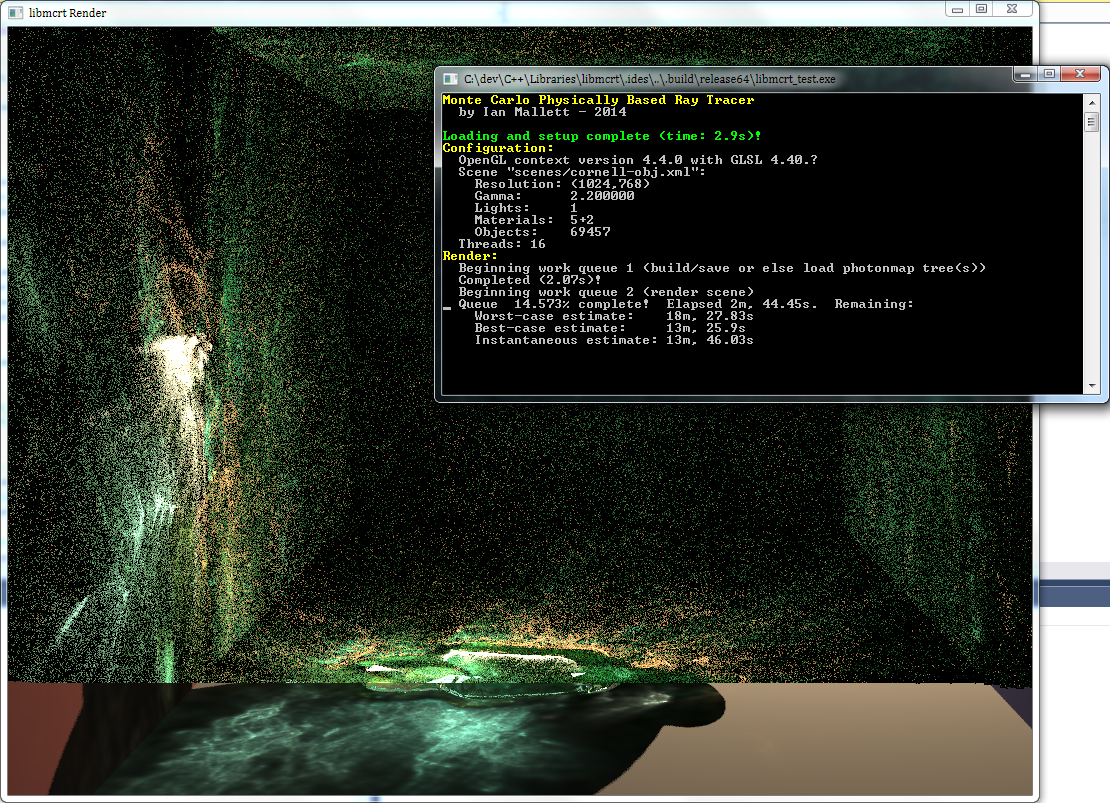
I strongly suspect that the slowest part is the photonmap traversal, since a Whitted render of the same scene to the same eye depth only takes a minute or so.

Proceed to the Previous Project or Next Project.

Hardware

Except as mentioned, renders are done on my laptop, which has:

• Intel i7-990X (12M Cache, [3.4{6|7},3.73 GHz], 6 cores, 12 threads)
• 12 GB RAM (DDR3 1333MHz Triple Channel)
• NVIDIA GeForce GTX 580M
• 750GB HDD (7200RPM, Serial-ATA II 300, 16MB Cache)
• Windows 7 x86-64 Professional (although all code compiles/runs on Linux)