CS 6620.001 "Ray Tracing for Graphics" Fall 2014
Welcome to my ray tracing site for the course CS 6620.001, being taught at the University of Utah in Fall 2014 by Cem Yuksel.
Welcome fellow students! I have lots of experience tracing rays, and with graphics in general, and so I'll be pleased to help by giving constructive tips throughout (and I'll also try very hard to get the correct image, or say why particular images are correct as opposed to others). If you shoot me an email with a link to your project, I'm pretty good at guessing what the issues in raytracers are from looking at wrong images.
Hardware specifications, see bottom of page.
Timing information will look like "(#t #s ##:##:##)" and corresponds to the number of threads used, the number of samples (per pixel, per light, possibly explained in context), and the timing information rounded to the nearest second.
Project 6 - "Space Partitioning"
Recall that these updates are mainly lame placeholders that satisfy requirements while I'm implementing several large new features. See project four for pretty pictures.
Recall the image from project five. This image rendered in a matter of seconds using my BVH implementation. Rather than wait for my tracer to finish tracing without an acceleration datastructure, I'm going to repost the \(10\) samples/pixel image from project four and give an extrapolation from what my renderer predicted the total time will be without the datastructure (based on rendering \(~0.50\%\) of the image). In reality, since the pixels that were rendered for the extrapolation comprised only simple shading, the timing would probably be somewhat longer.
My BVH is extremely dumb. Algorithmically:
- Bound every primitive with an AABB and find the center of that AABB.
- Make a root node.
- Make a collection of all the bounded objects.
- Set the current node to be the root node, and set its collection to be the collection of all bounded objects.
- Take the current node:
- If the current node's collection of bounded objects contains just one object, add it to the node itself. Otherwise, follow substeps \(2\) through \(7\):
- Bound the node's collection of bounded objects by a new AABB.
- Find the longest axis of that AABB. Sort the node's collection by their centers along that axis.
- Push the current node. Set the new current node to be a newly allocated child node of the old current node.
- Add half the collection of objects to the new current node's collection.
- Goto-with-return to step \(5\).
- Pop the current node. Repeat substeps \(4\), \(5\), and \(6\) with the other half of the objects.
I also implemented an octree, which is substantially smarter (although it's a worse datastructure). You basically just add objects into it and it subdivides itself iff it can separate at least two elements in a node. There are some tricks to make the building algorithm run in linear time. In retrospect, I think the renders below used a maximum depth of \(5\).
The project five image (rendered using a BVH):
The timing results for the different datastructures:
- BVH: (16t 10s 00:01:20)
- Octree: (16t 10s 00:02:35)
- None (estimated): (16t 10s 10:45:00)
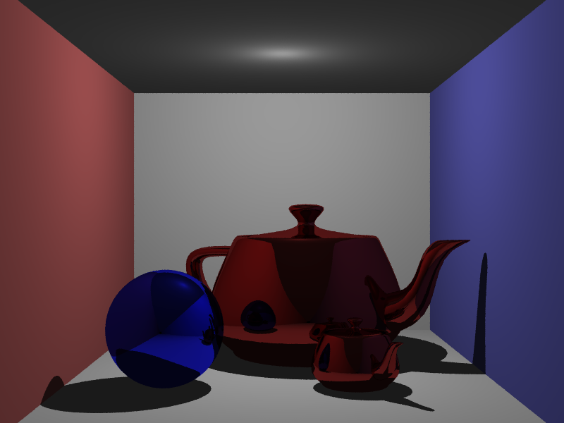
Here are some heatmaps of the acceleration datastructures running. "Scalar" is the amount the visualization parameter is scaled before the range \([0.0,1.0)\) is converted to the heatmap.
| Visualization | Scalar | BVH | Octree |
|---|---|---|---|
| Combination Operations/Primitives: Combines the cost of traversing the tree and of testing the primitives for the primary ray. The cost of traversing the tree is assumed to be the same as the number of ray-box intersections required. It is also possible to integrally scale the importance of each to the final sum, but here they both have weight \(1\). Of these visualizations, this is probably the best estimator of performance. | \(0.004\) | (16t 10s 00:00:02)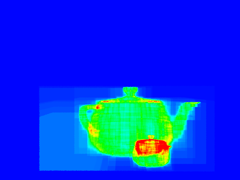 | (16t 10s 00:00:03)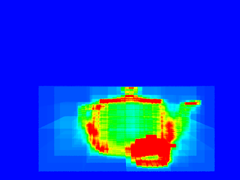 |
| Maximum Depth: Ignores primitive intersections; computes the deepest level of the datastructure along the primary ray. | \(0.06\) | (16t 10s 00:00:16)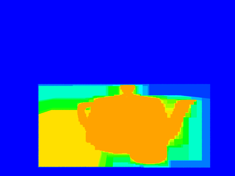 | (16t 10s 00:00:01)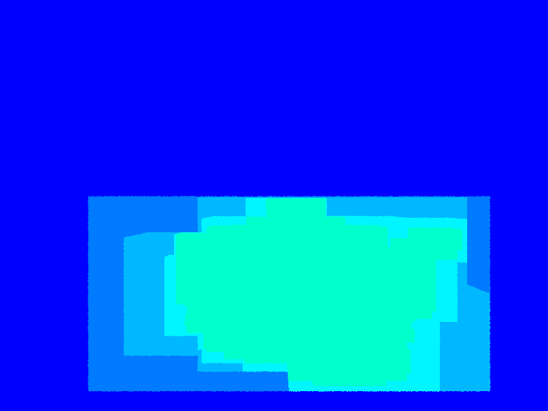 |
| Ray-Primitives: Counts the number of ray-primitive intersections. | \(0.06\) | (16t 10s 00:00:16)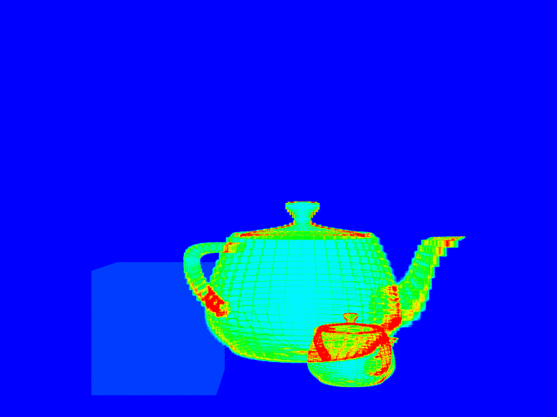 | (16t 10s 00:00:03)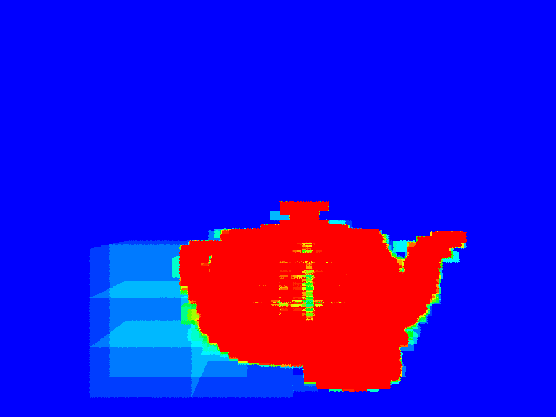 |
| Datastructure Operations: Counts the number of datastructure operations (ray-box intersections). | \(0.01\) | (16t 10s 00:00:02)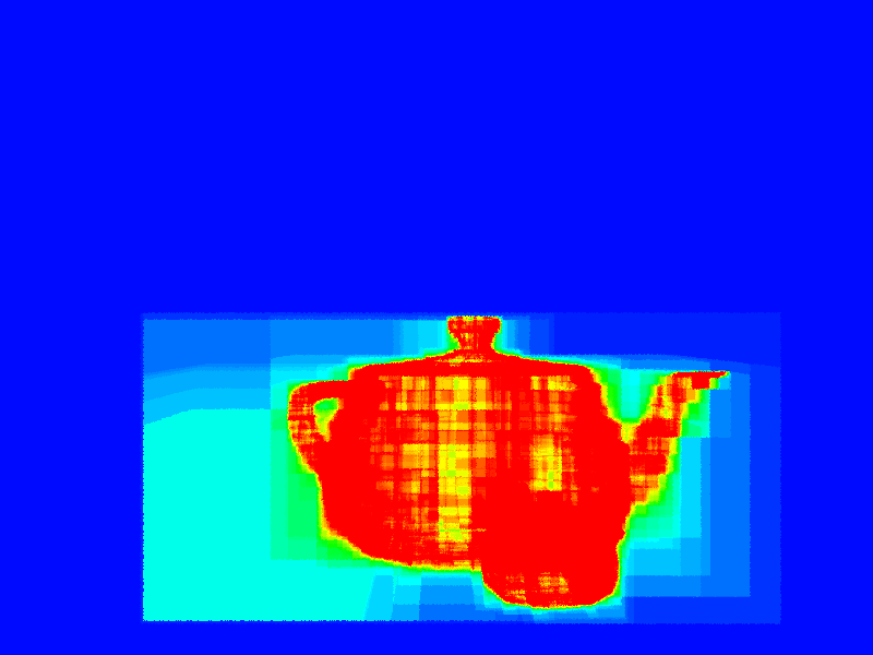 | (16t 10s 00:00:03)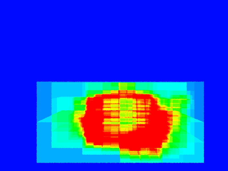 |
Of note is that the acceleration datastructures are brute force in the sense that they don't terminate early if a ray-primitive intersection is found. This is terrible.
After doing some other things (see project \(6.5\)), I came back and fixed it. The octree maximum depth here is \(10\). Here's some revised pictures:
| Visualization | Scalar | BVH | Octree |
|---|---|---|---|
| Combination Operations/Primitives: (As above) | \(0.001\) | (16t 10s 00:00:39)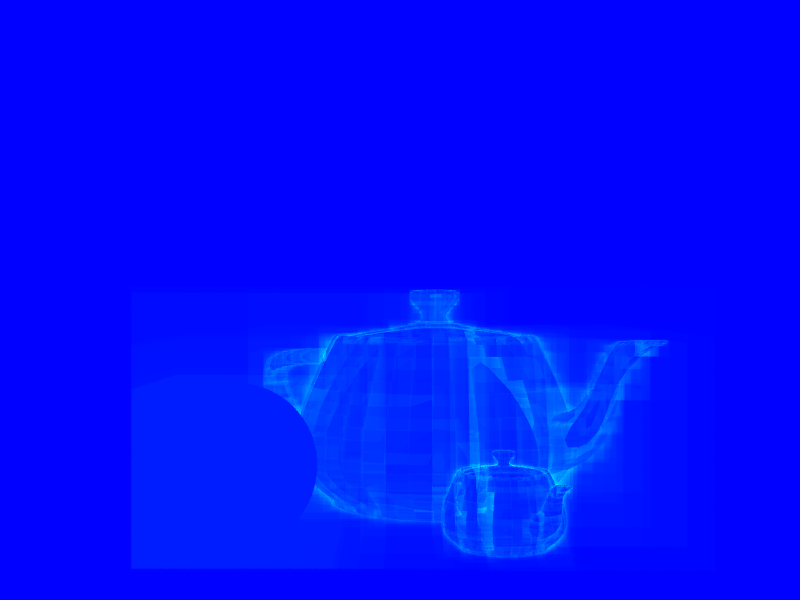 | (16t 10s 00:00:14)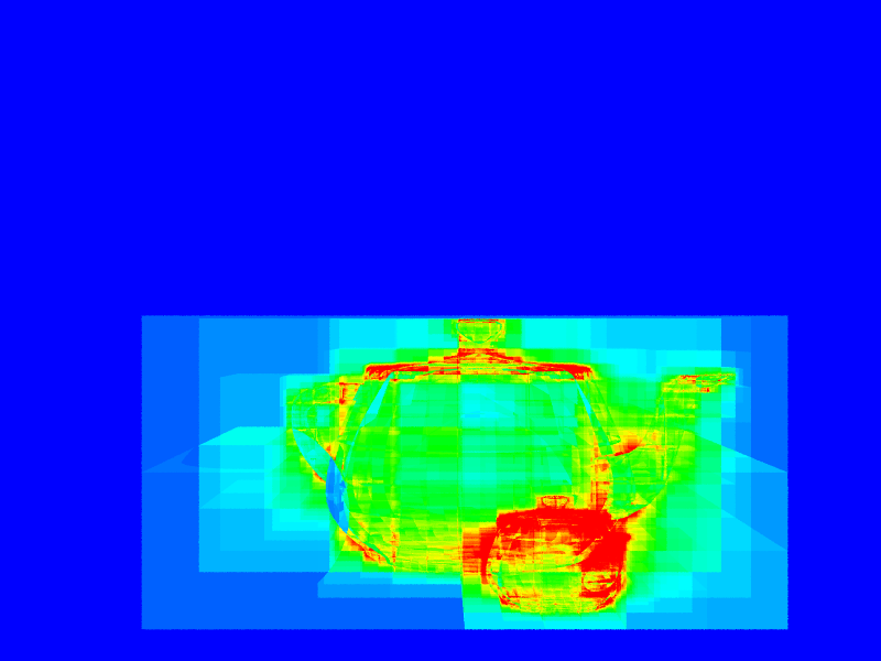 |
| Maximum Depth: (As above) | \(0.01\) | (16t 10s 00:00:14) | (16t 10s 00:00:32) |
| Ray-Primitives: (As above) | \(0.01\) | (16t 10s 00:00:13)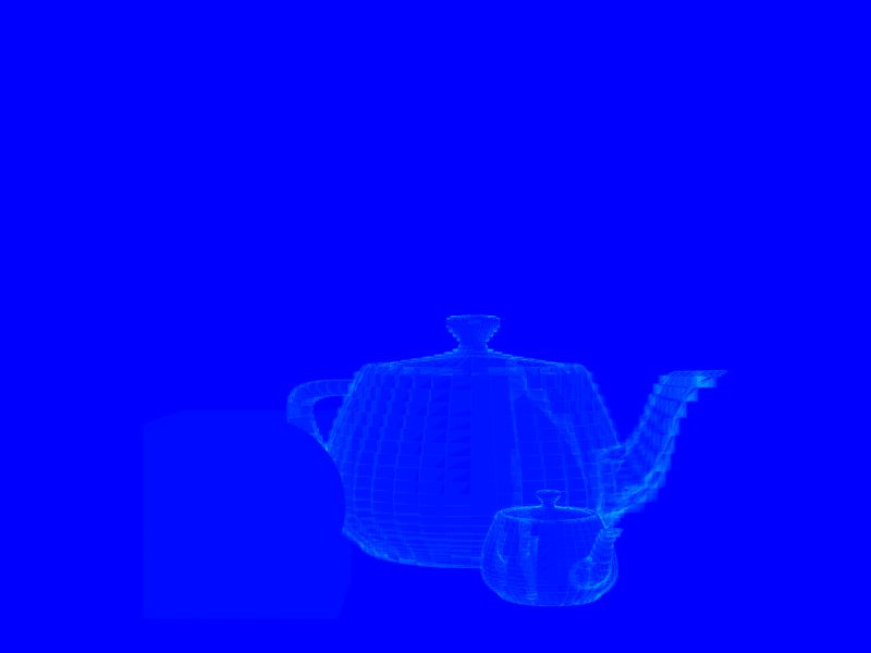 | (16t 10s 00:00:41)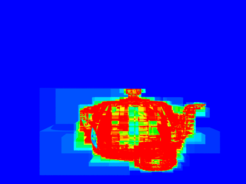 |
| Datastructure Operations: (As above) | \(0.001\) | (16t 10s 00:00:14) | (16t 10s 00:00:42)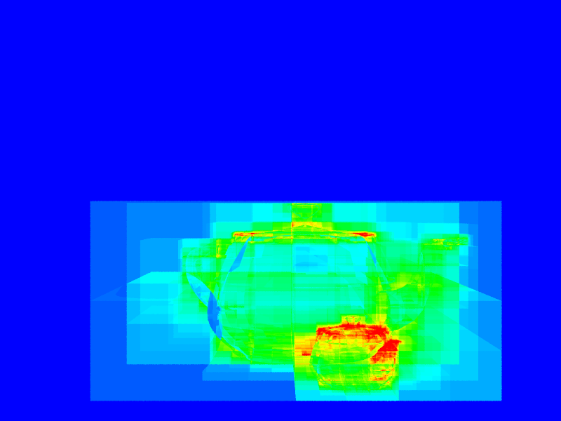 |
I later made a tweak to both datastructures that should improve performance. It's not worth redoing the above experiments.
Proceed to the Previous Project or Next Project.
Hardware
Except as mentioned, renders are done on my laptop, which has:
- Intel i7-990X (12M Cache, [3.4{6|7},3.73 GHz], 6 cores, 12 threads)
- 12 GB RAM (DDR3 1333MHz Triple Channel)
- NVIDIA GeForce GTX 580M
- 750GB HDD (7200RPM, Serial-ATA II 300, 16MB Cache)
- Windows 7 x86-64 Professional (although all code compiles/runs on Linux)